Jobs & Careers
Noida’s Suhora Brings Hyperspectral Satellite Services to India with Orbital Sidekick

Noida-based Suhora Technologies has partnered with US-based Orbital Sidekick (OSK) to launch high-resolution hyperspectral satellite services in India. The collaboration makes Suhora the first Indian company to offer commercial operational hyperspectral data across the visible and short-wave infrared (VNIR-SWIR) spectrum.
Under this agreement, Suhora will integrate OSK’s hyperspectral data into its flagship SPADE platform, enabling detailed material detection and classification. The service will support applications in mining, environmental monitoring, and strategic analytics.
Krishanu Acharya, CEO and co-founder of Suhora Technologies said, “This partnership with Orbital Sidekick marks an important step for the global geospatial community. The strategic applications enabled by this collaboration stand to benefit users globally, including India.”
Rupesh Kumar, CTO and co-founder, added that this addition will allow “precise mineral mapping, real-time environmental monitoring and anomaly detections.”
Suhora’s SPADE, a subscription-based SaaS platform, currently aggregates data from SAR, Optical, and Thermal satellites. With OSK’s hyperspectral data, SPADE will offer up to 472 contiguous spectral bands at 8.3-metre spatial resolution.
These capabilities will aid in applications such as rare earth mineral mapping, oil spill detection, and methane leak monitoring.
Suhora will leverage OSK’s GHOSt constellation of five satellites, which provide high revisit rates and full VNIR-SWIR coverage. The partnership is expected to deliver better temporal frequency and more precise data than other global providers like EnMAP, PRISMA, and NASA’s EMIT.
Tushar Prabhakar, co-founder and COO of Orbital Sidekick, commented, “Suhora’s strong local presence and expertise will be instrumental in delivering these powerful insights and driving significant value for our clients.”


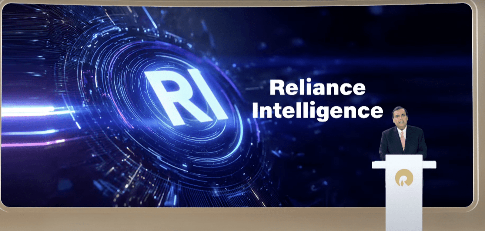
Reliance Industries chairman Mukesh Ambani has announced the launch of Reliance Intelligence, a new wholly owned subsidiary focused on artificial intelligence, marking what he described as the company’s “next transformation into a deep-tech enterprise.”
Addressing shareholders, Ambani said Reliance Intelligence had been conceived with four core missions—building gigawatt-scale AI-ready data centres powered by green energy, forging global partnerships to strengthen India’s AI ecosystem, delivering AI services for consumers and SMEs in critical sectors such as education, healthcare, and agriculture, and creating a home for world-class AI talent.
Work has already begun on gigawatt-scale AI data centres in Jamnagar, Ambani said, adding that they would be rolled out in phases in line with India’s growing needs.
These facilities, powered by Reliance’s new energy ecosystem, will be purpose-built for AI training and inference at a national scale.
Ambani also announced a “deeper, holistic partnership” with Google, aimed at accelerating AI adoption across Reliance businesses.
“We are marrying Reliance’s proven capability to build world-class assets and execute at India scale with Google’s leading cloud and AI technologies,” Ambani said.
Google CEO Sundar Pichai, in a recorded message, said the two companies would set up a new cloud region in Jamnagar dedicated to Reliance.
“It will bring world-class AI and compute from Google Cloud, powered by clean energy from Reliance and connected by Jio’s advanced network,” Pichai said.
He added that Google Cloud would remain Reliance’s largest public cloud partner, supporting mission-critical workloads and co-developing advanced AI initiatives.
Ambani further unveiled a new AI-focused joint venture with Meta.
He said the venture would combine Reliance’s domain expertise across industries with Meta’s open-source AI models and tools to deliver “sovereign, enterprise-ready AI for India.”
Meta founder and CEO Mark Zuckerberg, in his remarks, said the partnership is aimed to bring open-source AI to Indian businesses at scale.
“With Reliance’s reach and scale, we can bring this to every corner of India. This venture will become a model for how AI, and one day superintelligence, can be delivered,” Zuckerberg said.
Ambani also highlighted Reliance’s investments in AI-powered robotics, particularly humanoid robotics, which he said could transform manufacturing, supply chains and healthcare.
“Intelligent automation will create new industries, new jobs and new opportunities for India’s youth,” he told shareholders.
Calling AI an opportunity “as large, if not larger” than Reliance’s digital services push a decade ago, Ambani said Reliance Intelligence would work to deliver “AI everywhere and for every Indian.”
“We are building for the next decade with confidence and ambition,” he said, underscoring that the company’s partnerships, green infrastructure and India-first governance approach would be central to this strategy.
The post ‘Reliance Intelligence’ is Here, In Partnership with Google and Meta appeared first on Analytics India Magazine.

Cognizant has announced that it would deploy 1,000 context engineers over the next year to industrialise agentic AI across enterprises.
According to an official release, the company claimed that the move marks a “pivotal investment” in the emerging discipline of context engineering.
As part of this initiative, Cognizant said it is partnering with Workfabric AI, the company building the context engine for enterprise AI.
Cognizant’s context engineers will be powered by Workfabric AI’s ContextFabric platform, the statement said, adding that the platform transforms the organisational DNA of enterprises, how their teams work, including their workflows, data, rules, and processes, into actionable context for AI agents.Context engineering is essential to enabling AI a
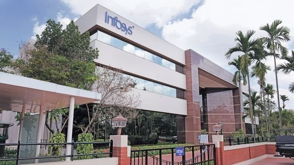
Infosys has announced a partnership with Mastercard to make cross-border payments faster and easier for banks and financial institutions.
The collaboration will give institutions quick access to Mastercard Move, the company’s suite of money transfer services that works across 200 countries and over 150 currencies, reaching more than 95% of the world’s banked population.
Sajit Vijayakumar, CEO of Infosys Finacle, said, “At Infosys Finacle, we are committed to inspiring better banking by helping customers save, pay, borrow and invest better. This engagement with Mastercard Move brings together the agility of our composable banking platform with Mastercard’s unmatched global money movement capabilities—empowering banks to deliver fast and secure cross-border experiences for every customer segment.”
Integration will be powered by Infosys Finacle, helping banks connect with Mastercard’s system in less time and with fewer resources than traditional methods.
Pratik Khowala, EVP and global head of transfer solutions at Mastercard, said, “Through Mastercard Move’s cutting-edge solutions, we empower individuals and organisations to move money quickly and securely across borders.”
The tie-up also comes at a time when global remittances are on the rise. Meanwhile, Anouska Ladds, executive VP of commercial and new payment flows, Asia Pacific at Mastercard, noted, “Global remittances continue to grow, driven by migration, digitalisation and economic development, especially across Asia, which accounted for nearly half of global inflows in 2024.”
He further said that to meet this demand, Mastercard invests in smart money movement solutions within Mastercard Move while expanding its network of collaborators, such as Infosys, to bring the benefits to a more diverse set of users.
Infosys said the partnership will help banks meet growing consumer demand for faster and safer payments.
Dennis Gada, EVP and global head of banking and financial services at Infosys, said, “Financial institutions are prioritising advancements in digital payment systems. Consumers gravitate toward institutions that offer fast, secure and seamless transaction experiences. Our collaboration with Mastercard to enable near real-time, cross-border payments is designed to significantly improve the financial experiences of everyday customers.”
The post Mastercard, Infosys Join Hands to Enhance Cross-Border Payments appeared first on Analytics India Magazine.
-
Tools & Platforms3 weeks ago
Building Trust in Military AI Starts with Opening the Black Box – War on the Rocks
-
 Ethics & Policy1 month ago
SDAIA Supports Saudi Arabia’s Leadership in Shaping Global AI Ethics, Policy, and Research – وكالة الأنباء السعودية
-

 Events & Conferences3 months ago
Journey to 1000 models: Scaling Instagram’s recommendation system
-

 Jobs & Careers2 months ago
Mumbai-based Perplexity Alternative Has 60k+ Users Without Funding
-

 Business1 day ago
The Guardian view on Trump and the Fed: independence is no substitute for accountability | Editorial
-

 Funding & Business2 months ago
Kayak and Expedia race to build AI travel agents that turn social posts into itineraries
-
 Education2 months ago
VEX Robotics launches AI-powered classroom robotics system
-

 Podcasts & Talks2 months ago
Happy 4th of July! 🎆 Made with Veo 3 in Gemini
-

 Podcasts & Talks2 months ago
OpenAI 🤝 @teamganassi
-

 Jobs & Careers2 months ago
Astrophel Aerospace Raises ₹6.84 Crore to Build Reusable Launch Vehicle