Here we delve into the implementation of proactive trajectory modulation as a means of slip control, which addresses our first hypothesis. We present the methodology and experimental setup used to examine the effectiveness of trajectory modulation in preventing slip incidents during robotic manipulation tasks. Furthermore, we introduce the concept of incorporating a forward model in proactive control, an approach aimed at slip avoidance, as per our second research hypothesis. We outline the key aspects of proactive control, its implementation and the experimental framework used to evaluate its performance in slip prevention.

Experimental setup

Traditional parallel jaw grippers are still widely used in many robotic manipulation tasks, such as bin picking ³⁸. Usually, a motion planning module generates a reference trajectory for the robot by minimizing, for example, time or jerk before motion execution. Then, the robot executes them in an open-loop manner with respect to task failure/success due to a slip in real time. This limits the robot’s success, and solutions in the literature suggest increased grip force on the fly, which may not be feasible in many cases^39,40,41. We address this issue using our data-driven predictive control concept, referred to as proactive control.

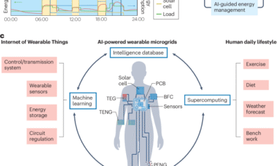
First, we collected a dataset of open-loop trajectory executions in which the robot manipulates an object included in our train objects set shown in Supplementary Table 2. We equipped the fingers of a Franka Emika robotic arm with a pair of 4 × 4 uSkin tactile sensors and performed moving tasks with multiple objects. The uSkin tactile sensor has 16 sensing points (taxels) that measure triaxial forces, including shear x, shear y and normal z (Fig. 1). To create various types of reference trajectory, we used two main motion strategies during data collection: (1) kinaesthetic robot motions, where a human user performed moving tasks with qualitative fast and slow motions; (2) automatic robot motions, where trapezoidal reference trajectories with various acceleration/deceleration values were sent as a reference Cartesian velocity. A D435i camera manufactured by Intel RealSense mounted on the robot’s wrist measures the pose of an ArUco marker attached to the top of the object. The pose data are then post-processed to create binary slip labels based on the object’s in-hand displacement.

ACTP

In this work, tactile data are referred to as frames, representing single time-step readings of the respective sensing modality. Given (1) a set of context frames f_0:c−1 = {f₀…f_c−1}, which are the previously observed frames with a context sequence length of c, and (2) a prediction horizon of length H – c (that is, the number of future frames to predict); here we assume equal context and prediction window size, that is, H = 2c, where \({i}_{c}\in \{0,\ldots ,c-1\}\in {{\mathbb{Z}}}^{c}\), \({i}_{p}\in \{c,\ldots ,H-1\}\in {{\mathbb{Z}}}^{c}\) and \(i\in \{0,\ldots ,c-1\}\cup \{c,\ldots ,H-1\}\in {{\mathbb{Z}}}^{H}\) (Fig. 3b shows details of the samples in the context and prediction horizons). Although here we show the formulation for one time step f(t), generalization for training for the entire trajectory, that is, t = 0:T, is straightforward. A tactile prediction model can be defined as f (we use *_i:i+n = {*_i, *_i+1…*_i+n}; Fig. 3b) to denote variables representing the set of frames and \(\hat{{\bf{f}}}\) to denote the corresponding predicted values:

where \({\hat{{\bf{f}}}}_{c:H-1}\) represents a set of predicted frames \({\hat{{\bf{f}}}}_{i}\in {{\mathbb{R}}}^{48}\) (tactile images). The goal is to optimize equation (2), for each time step in the prediction horizon counted by i_p:

where \({\mathcal{D}}\) denotes the loss function in the tactile reading space or pixel space, such as \({{\mathcal{L}}}_{1}\) or \({{\mathcal{L}}}_{2}\), measuring the difference between the predicted and observed frames.

In a physical robot interaction, we aim to develop a cause–effect understanding of the robot’s actions. Thus, we condition the prediction model on the past context frames f_0:c−1, the past robot trajectory x_0:c−1 and planned robot actions a_c−1:H−2 to output future frames \({\hat{{\bf{f}}}}_{c:H-1}\) (which are known in our physical robot interaction datasets but unknown during the inference time). Here \({{\bf{x}}}_{{i}_{c}}\in {{\mathbb{R}}}^{6}\) represents the robot trajectory at past steps, and \({{\bf{a}}}_{{i}_{p}}\in {{\mathbb{R}}}^{6}\) represents the planned future robot actions at time t. The model assumes a known and nearly constant sampling frequency (typically around 10 Hz with less than 10% variance), and we work with discrete values. The prediction model can be expressed as

where f denotes tactile frames. In model predictive control, which commonly uses forward prediction models like those described here, future robot actions are considered as a batch of candidate actions. The optimal action is selected by a discriminator based on the most desirable predicted tactile frames^34,42.

Our model aims to maximize the \(p\left(\right.{\hat{{\bf{f}}}}_{c:H-1}| {{\bf{f}}}_{0:c-1},\)\(\{{{\bf{x}}}_{0:c-1},{{\bf{a}}}_{c-1:H-2}\},\) \(\left.{{\bf{z}}}_{0:c}\right)\) to predict tactile frame \({\hat{{\bf{f}}}}_{c:T}\) by applying stochastic assumption to the prediction model. Our objective is to sample from

The network can then be trained with the frame prediction model by maximizing equation (4).

For more information about action-conditioned prediction models, see refs. ^35,43,44. The LSTM classifier takes the predicted tactile frames and classifies each predicted time step as either slip or non-slip. The resulting slip signal, where the binary value of 0 indicates no slip and 1 indicates slip, is then used in the model predictive control framework to adjust the robot’s movements accordingly.

Slip classification model

To classify tactile frames as slip and non-slip signals, we leverage the temporal processing capabilities of LSTM networks, which have been shown to significantly enhance the classification performance by incorporating historical tactile features, compared with traditional classification methods such as support vector machines^45,46.

Formally, we define the slip classification task as mapping the predicted tactile state sequence \({\hat{{\bf{f}}}}_{c:H-1}\) to a sequence of slip classifications \({\hat{{\bf{s}}}}_{c:H-1}\), where each \({\hat{{\bf{s}}}}_{i}\in \{{c}_{{\text{slip}}},{c}_{{\text{non-slip}}}\}\) denotes the slip status at time step i within the prediction window. The LSTM model is trained to learn the temporal dependencies in the tactile data, enabling it to effectively differentiate between slip and non-slip conditions.

Given a sequence of predicted tactile states \({\hat{{\bf{f}}}}_{c:H-1}\), the LSTM-based slip classifier processes these states sequentially, with the LSTM unit updates defined as follows:

where h_i and c_i are the hidden and cell states at time step i, respectively. The output of the LSTM at each time step is passed through a fully connected layer to produce the slip classification logits, which are then converted into probabilities using a sigmoid activation function:

where σ is the sigmoid function, and W_s and b_s are the weight and bias of the output layer, respectively. The final slip classification \({\hat{{\bf{s}}}}_{i}\) is obtained by thresholding the probability output, assigning it to either the slip or non-slip class.

The architecture of the LSTM-based slip classification model is depicted in Fig. 2. Building on the work in ref. ³⁴, which demonstrated that a simple LSTM-based tactile forward model combined with a slip classifier outperforms classifiers labelled with future slip instances, we use a state-of-the-art tactile forward model³⁵ to estimate tactile states over the future prediction horizon and classify these predicted states accordingly.

To determine the stability of the object in the robot’s grip, the slip classification model primarily utilizes the shear force components from the predicted tactile states. To enhance the model’s generalization ability, we incorporate two dropout layers with a dropout probability of 0.5.

The slip classification dataset is imbalanced, comprising 16% slip instances and 84% non-slip instances. To address this imbalance, we train the classification model using the binary cross-entropy loss function, with a weighting scheme that penalizes slip instances more heavily than non-slip cases, using a relative weight of 3:1. This approach helps ensure that the classifier is conservative, with a strong tendency to predict actual slip instances as positive, leading to high recall rates, as reflected in the metrics in Supplementary Table 1 (right) for most of the train and test objects.

Slip control using trajectory modulation

Our proactive control approach, based on our previous work³⁴, consists of a tactile forward model, a slip classifier and a predictive controller. A detailed presentation of model architecture and hyperparameters settings of ACTP and the slip classification models is included in Supplementary Section 1. We have made several improvements to the original approach that have led to substantial performance gains. First, we have incorporated our ACTP model to improve the accuracy of the slip classifier (Supplementary Table 1 provides the results). Second, we have extended the control variable from one DOF to six DOFs. This control strategy regulates the distance to the reference trajectory (which we call residual values), rather than learning the Cartesian velocity, as that in ref. ⁴⁷. This results in improved optimization and better convergence and generalization. Additionally, we have expanded the object and trajectory sets, further improving the generalization of the approach. We denote the Cartesian-space velocity vector of the robot as \(\overrightarrow{V}=({V}_{x},{V}_{y},{V}_{z},\,{W}_{x},{W}_{y},{W}_{z})\).

In the trajectory modulation loop, the first three components of the control vector represent the translational velocities along the Cartesian coordinate axes, whereas the last three components represent the angular velocities around those axes. Our goal is to minimize the future slip likelihood \(L({s}_{c,\ldots ,H-1}| \alpha ,\beta ,{\bf{x}},{\bf{a}})=\mathop{\prod }\nolimits_{i = c}^{H-1}f({s}_{i}| \alpha ,\beta ,{{\bf{x}}}_{0:i},{{\bf{a}}}_{i})\) by learning the optimal deviation from the reference velocity profile, where α, β, x and a represent the tactile forward model and slip classifier parameters, past tactile states and planned robot actions, respectively. s_i indicates the ith observed slip value within a prediction horizon of length c. We choose spherical coordinates as the robot’s input {a_c−1…a_H−2} to adapt a given reference trajectory. As such, we modify the reference velocity vector by separately adjusting its norm and direction. To facilitate this modification, we represent the translational and angular velocities in spherical coordinates as follows.

The variables ρ, θ and ϕ correspond to the norm, polar angle and azimuthal angle, respectively, in spherical coordinates. The relationship between the spherical and rectangular coordinates is illustrated in Extended Data Fig. 1. Using spherical coordinates enables the optimization process to separately learn the modifications needed for the norm and direction of the velocity vector in space. The optimization process returns the residual values, which are added to the components in equation (8) to modify the reference velocity profile.

We express the residual values of equation (9) in the matrix form as \({\zeta }^{{\rm{d}}}=({\zeta }_{{\rho }_{v}},{\zeta }_{{\theta }_{v}},{\zeta }_{{\phi }_{v}},{\zeta }_{{\rho }_{w}},{\zeta }_{{\theta }_{w}},{\zeta }_{{\phi }_{w}})\). The residual trajectory values form the difference between the executed robot trajectory ζ^e and the reference trajectory ζ^r are \({\zeta }_{c:H-1}^{\;{\rm{d}}}={\zeta }_{c:H-1}^{\;{\rm{e}}}-{\zeta }_{c:H-1}^{\;{\rm{r}}}\) and \({\zeta }_{c:H-1}^{{\rm{e}}}=\{{{\bf{a}}}_{c-1}\ldots {{\bf{a}}}_{H-2}\}\), where \({\bf{a}}\in {{\mathbb{R}}}^{6}\) and \(\zeta \in {{\mathbb{R}}}^{6\times c}\).

Parameterized residual learning for trajectory adaptation

To optimize the robot’s trajectories over a future time horizon (that is, \({i}_{{\rm{p}}}\in \{c,\ldots H-1\}\in {{\mathbb{Z}}}^{c}\)), we represent the residual values using a parametric action representation⁴⁸ that includes a weight parameter matrix w to be computed by the optimizer using Gaussian basis functions⁴⁹, which is denoted by Φ: \({\zeta }_{c:H-1}^{\;{\rm{d}}}={{\bf{w}}}^{{\rm{T}}}\times \varPhi\), where \(\varPhi \in {{\mathbb{R}}}^{n\times c}\) and \({\bf{w}}\in {{\mathbb{R}}}^{c\times 6}\). For the sake of simplicity, we express ζ_c:H−1 by ζ.

The parameterized action space representation reduces computation complexity compared with direct search in continuous action space⁴⁸. The benefit is more effective when the action is optimized in a future time horizon rather than a single time step due to the fewer search parameters in the optimization problem. We close the loop for the slip prevention controller by solving the constraint optimization in equation (10).

where ζ^e = ζ^d(w, Φ) + ζ^r, and f denotes the tactile state vector \(\in {{\mathbb{R}}}^{48\times c}\). The first nonlinear constraint in the optimization formulation is based on the expected value of the slip signal over the prediction horizon c, given by \({\mathbb{E}}[{s}_{c:H-1}({\zeta }^{{\rm{e}}}({\bf{w}},\varPhi ))]\), where s is a function of the robot’s future trajectory. The second constraint limits the difference between the generated robot velocities and the observed velocity (measurement) to ensure compliance with the robot’s low-level controller maximum acceleration limit. The optimization problem seeks to minimize the expected slip over the prediction horizon and remaining close to the provided reference trajectory.

The resulting spherical velocity components are transformed back to rectangular coordinates before being sent to the robot’s Cartesian-velocity controller as per equation (11). The V_x, V_y, V_z, W_x, W_y and W_z values are used to update the robot’s Cartesian-velocity controller, which regulates the robot’s motion along the desired trajectory and avoiding slipping.

We provide a detailed presentation of the grip force control method as the baseline controller for benchmarking our proactive controller in the Supplementary Information.

Training and testing

We trained our ACTP model and slip classification model offline using a dataset of pick-and-move tasks. Figure 2 illustrates the forward model and its architecture within a predictive control pipeline⁵⁰.

The manipulation dataset consists of 420,000 data samples collected from 600 manipulation trials involving 13 box-shaped objects. Each object (including both train and test set objects; Supplementary Tables 1 and 2 list the dataset details) was involved in an equal number of trials, with three objects reserved as test objects, which were not seen during training. The performance of the ACTP and slip classification models was validated by analysing the mean absolute error and F-score values for the unseen objects, respectively. All models were trained on a Ubuntu machine equipped with an AMD Ryzen Threadripper CPU, NVIDIA GeForce RTX 2080 GPU and 64 GB of memory. The training was conducted using the PyTorch v. 1.13.1 library with CUDA v. 11.7. The trained ACTP and slip classification models are then used with fixed-weight parameters for real-time control tests.

During testing, the trajectory modulation module utilizes the inference from these two models in an online optimization loop to determine the optimal next robot action that minimizes the likelihood of slip occurrence in a receding horizon framework. We will now present the design details for each building block of the proactive control system (Fig. 2).

Objects, metrics and comparison method

Table 2 presents the objects used for training and testing our controller (Supplementary Table 1 provides the pictures of each object). It also details the performance metrics for both train and test objects. The train and test sets are based on the data collection for training the underlying tactile forward model and slip classifier in the proactive control, consisting of ten train objects and three test objects. The performance metrics for the slip controller include rotation of >6°, time steps (RTS) and maximum object rotation (MOR) in degrees. RTS represents the number of time steps during which the object’s rotation exceeded the slip classification threshold (6°). Smaller RTS values indicate better slip avoidance performance. The proactive control achieved excellent performance with no slip instances (RTS = 0) for five objects in the train set and two objects in the test set (boldface values in the RTS column). The MOR values show that for five objects, the maximum rotation slightly exceeded 6°, the threshold set for slip classification. This may be attributed to the imprecision of the forward model, the classifier (Supplementary Table 1) or the threshold we set on the number of iterations in the controller computations to find the optimal actions (as we allow only ten optimizer iterations due to real-time constraints). Nonetheless, MOR remains below 9°, preventing failure despite slip instances. Comparing the mean values of MOR and RTS for the train and test sets demonstrates that our proposed controller generalizes well to unseen objects during training and effectively avoids slip instances on average. DRT denotes the distance to the reference trajectory, calculated by summing the Euclidean distance between the reference and optimized trajectories across all task time steps (measured in m s⁻¹). ROV represents the resulted optimality value, indicating the convergence of the optimization process at the final iteration.

Reporting summary

Further information on research design is available in the Nature Portfolio Reporting Summary linked to this article.