Events & Conferences
Automated reasoning at Amazon: A conversation

The Federated Logic Conference (FLoC) is a superconference that, like the Olympics, happens every four years. FLoC draws together 12 distinct conferences on logic-related topics, most of which meet annually. The individual conferences have their own invited speakers, but FLoC as a whole has several plenary speakers as well.
At the last FLoC, in 2018, one of those plenary speakers was Byron Cook, who leads Amazon’s automated-reasoning group, and he was introduced by Daniel Kröning, then a professor of computer science at the University of Oxford
Byron Cook’s keynote at FLoC 2018
With introduction by Daniel Kröning.
“What makes me so proud that Byron is here,” Kröning said, is “he’s now at Amazon, and he’s going to run the next Bell Labs, he’s going to run the next Microsoft Research, from within Amazon. My prediction is that — not 10 years but 16 years; remember, it’s multiples of four — 16 years from now you’ll be at a FLoC, and you’ll hear these stories about the great thing that Byron Cook built up at Amazon Web Services. And we’ll speak about it in the same tone as we’re now talking about Bell Labs and Microsoft Research.”
In the audience at the talk was Marijn Heule, a highly cited automated-reasoning researcher who was then at the University of Texas.
“I hadn’t met Marijn, though I had heard about him from a couple other people and thought I should talk to him,” Cook says. “And then Marijn found me at the banquet after the talk and was like, ‘I want a job.’”
Heule is now an Amazon Scholar who divides his time between Amazon and his new appointment at Carnegie Mellon University. Kröning, too, has joined Amazon as a senior principal scientist, working closely with Cook’s group.
As 2022’s FLoC approached, Cook, Kröning, and Heule took some time to talk with Amazon Science about the current state of automated-reasoning research and its implications for Amazon customers.
Amazon Science: The conference name has the word “logic” in it. Does FLoC deal with other aspects of logic, or is logic coextensive with automated reasoning now?
Byron Cook: It’s about the intersection of logic and computer science. Automated reasoning is one dimension of that intersection.
Daniel Kröning: Traditionally, FLoC is split into two halves, with the first half more theoretical and the second half more applied.
Cook: One of the things about automated reasoning is you’re on the bleeding edge of what is even computable. We’re often working on intractable or undecidable problems. So people automating reasoning are really paying attention to both the applied and the theoretical.
AS: I know Marijn is concentrating on SAT solvers, and SAT is an intractable problem, right? It’s NP-complete?
Marijn Heule: Yes, but you can also use these techniques to solve problems that go beyond NP. For example, solvers for SAT modulo theories, called SMT. I even have a project with one student trying to solve the famous Collatz conjecture with these tools.
Kröning: SAT is now the inexpensive, easy-to-solve workhorse for really hard problems. People still have it in their heads that SAT equals NP hard, therefore difficult to solve or impossible to solve. But for us, it’s the lowest entry point. On top of SAT, we build algorithms for solving problems that are way harder.
Cook: One of the tricks of the trade is abstraction, where you take a problem that’s much, much bigger but represent it with something smaller, where classes of questions you might ask about the smaller problem imply that the answer also holds for the bigger problem. We also have techniques for refining the abstractions on demand when the abstraction is losing too much information to answer the question. Often we can represent these abstractions in tools for SAT.
Marijn’s work on the Collatz conjecture is a great example of this. He has done this amazing reduction of Collatz to a series of SAT questions, and he’s tantalizingly close to solving it because he’s got one decidable problem to go — and he’s the world expert on solving those problems. [Laughs]
Heule: Tantalizingly close but also so far away, right? Because this problem might not be solvable even with a million cores.
Cook: But it’s still decidable. And one of the thresholds is that NP, PSpace, all these things, they’re actually decidable. There are questions that are undecidable — and we work on those, too. When a problem is undecidable, it means that your tool will sometimes fail to find an answer, and that’s just fundamental: there are no extra computers you could use ever to solve that. The halting problem is a great example of that.
Heule: For these kinds of problems, you’re asking the question “Is there a termination argument of this kind of shape?” And if there is one, you have your termination argument. If there is no termination argument of that shape, there could be one of another shape. So if the answer is SAT [satisfiable], then you’re happy because you’ve solved the problem. If the answer is no, you try something else.
Cook: It’s really, really exciting. In Amazon, we’re building these increasingly powerful SAT solvers, using the power of the cloud and distributed systems. So there’s no better place for Marijn to be than at Amazon.
AS: Daniel, could we talk a little bit about your research?
Kröning: What I’m looking at right now is reasoning about the cloud infrastructure that performs remote management of EC2 instances — how to secure that in a way that is provable. You also want to do that in a way that is economical.
Cook: One of the things that Daniel’s focusing on is agents. We have pieces of software that run on other machines, like EC2 instances, agents for telemetry or for control, and you give them power to take action on your behalf on your machine. But you want to make sure that an adversary doesn’t trick those agents into doing bad things.
Correct software
AS: I know that, commercially, formal methods have been used in hardware design and transportation systems for some time. But it seems that they’re really starting to make inroads in software development, too.
The storage team is able to write code that otherwise they might not want to deploy because they wouldn’t be as confident about it, and they’re deploying four times as fast. It was an investment in agility that’s really paid off.
Cook: The thing we’ve seen is it’s really by need. The storage team, for example, is able to be much more agile and be much more aggressive in the programs that they write because of the formal methods. They’re able to write code that otherwise they might not want to deploy because they wouldn’t be as confident about it, and they’re deploying four times as fast. It was an investment in agility that’s really paid off.
Kröning: There are actually a good number of stories wherein engineering teams didn’t dare to roll out a particular feature or design revision or design variant that offers clear benefits — like being faster, using less power — because they just couldn’t gain the confidence that it’s actually right under all circumstances.
Heule: The interesting thing is that you even see this now in tools. Now we have produced proofs from the tools, and people start implementing features that they wouldn’t dare have in the past because they were not clear that they were correct. So the solvers get faster and more complex because we now can check the results from the tools and to have confidence in their correctness.

Cook: Yeah, I wanted to double down on that point. There’s a distinction in automated reasoning between finding a proof and checking your proof, and the checking is actually relatively easy. It’s an accounting thing. Whereas finding the proof is an incredibly creative activity, and the algorithms that find proofs are mind-blowing. But how do you know that the tool that found the proof is correct? Well, you produce an auditable artifact that you can check with the easy tool.
SAT in the cloud
AS: What are you all most excited about at this year’s FLoC?
Cook: The SAT conference is at FLoC, and there will be the SAT competition results, and one of the things I’m really excited about is the cloud track. Automated reasoning has really moved into the cloud, and the past couple years running the cloud track has really blown the doors off what’s possible. I’m expecting that that will be true again this year.
Heule: This is the first year that Amazon is running both the parallel track and the cloud track, and the cloud track was only possible because of Amazon. Before that, there was no way we had the resources to run a cloud track. In the cloud track, every solver-benchmark combination is run on 1,600 cores. And this year is extra special because it’s 20 years of SAT, and we have a single anniversary track and all the competitions that were run in the past are in there. That is 5,355 problems, and all the solvers are running on this.
Cook: Wow.
Heule: I’m also excited to see the results. We have seen in the last year and the year before that the cloud solver can, say, solve in 100 seconds as much as the sequential solvers can do in 5,000 seconds. The user doesn’t have to wait for four hours but just for four minutes
Cook: And that raises all boats because, as we mentioned earlier, everything is reduced to SAT. If the SAT solvers go from one hour to one minute, that’s really game changing. That means a whole other set of things you can do.
What has been clear for a while but continues to be true is there’s some sort of Moore’s-law thing happening with SAT. You fix the same hardware, the same benchmarks, and then run all the tools from the past 20 years, and you see every year they’re getting dramatically better. What’s also really amazing is that in many ways the tools are getting simpler.
LH: Are the simplicity and efficiency two sides of the same coin? Understanding the problems better helps you find a simpler solution, which is more efficient?
Cook: Yeah, but it’s also the point that Marijn made that because the tools produce auditable proofs that you can check independently, you can do aggressive things that we were scared to do before. Often, aggressive is much simpler.

Heule: It’s also the case that we now understand there are different kinds of problems, and they need different kinds of heuristics. Solvers are combining different heuristics and have phases: “Let’s first try this. Let’s also try that.” And the code involved in changing the heuristics is very small. It’s just changing a couple of parameters. But if you notice, okay, this set of heuristics works well for this problem, then you kind of focus more on that.
Cook: One of the things a SAT solver does is make decisions fast. It just makes a bunch of choices, and those choices won’t work out, and then it spends some time to learn lessons why. And then it has a very efficient internal database for managing what has been learned, what not to do in the future. And that prunes the search space a lot.
One of the really exciting things that’s happening in the cloud is that you have, say, 1,000 SAT solvers all running on the same problem, and they’re learning different things and can share that information amongst them. So by adding 5,000 more solvers, if you can make the communication and the lookup efficient between them, you’re really off to the races.
The other thing that’s quite neat about that is the point that Marijn is making: it’s becoming increasingly clear that there are these fundamental building blocks, and for different kinds of problems, you would want to use one kind of Lego brick versus a different kind of Lego brick. And the cloud allows you to run them all but then to share the information between them.
Heule: We have an Amazon paper at FLoC with some very cool ideas. If you run things in the cloud, you sometimes have a limited time window where you have to solve them, and otherwise it stops. You started with a certain problem, the solver did some modifications, and now we have a different problem. Initially we just tested, Okay, can we stop the solver and then store the modified problem somewhere and continue later, in case we need more time than we allocated initially? And then we can continue solving it.
But the interesting thing is that if you give the modified problem to another solver, and you give it, say, a couple of minutes, and then it stores the modified problem, and you give it to another solver, it actually really speeds things up. It turns out to solve the most instances from everything that we tried.
AS: Do you do that in a principled way, or do you just pick a new solver randomly?
Heule: The thing that turned out to work really well is to take two top-tier solvers and just Ping-Pong the problem among them. This functionality of storing and continuing search requires some work, so that implementing it in, say, a dozen solvers would require quite some work. But it would be a very interesting experiment.
AS: I’m sure our readers would love to know the result of that experiment!
Well, thank you all very much for your time. Does anyone have any last thoughts?
Cook: I think I speak for the thousands of others who are attending FLoC: we are ready to having our minds blown, just as we did in 2018. Many of the tools and theories presented by our scientific colleagues at this year’s FLoC will challenge our current assumptions or spark that next big insight in our brains. We will also get to catch up with old friends that we’ve known for around 20 years and meet new ones. I’m particularly excited to meet the new generation of scientists who have entered the field, to see the world afresh through their eyes. This is such an amazing time to be in the field of automated reasoning.


Modern warehouses rely on complex networks of sensors to enable safe and efficient operations. These sensors must detect everything from packages and containers to robots and vehicles, often in changing environments with varying lighting conditions. More important for Amazon, we need to be able to detect barcodes in an efficient way.
The Amazon Robotics ID (ARID) team focuses on solving this problem. When we first started working on it, we faced a significant bottleneck: optimizing sensor placement required weeks or months of physical prototyping and real-world testing, severely limiting our ability to explore innovative solutions.
To transform this process, we developed Sensor Workbench (SWB), a sensor simulation platform built on NVIDIA’s Isaac Sim that combines parallel processing, physics-based sensor modeling, and high-fidelity 3-D environments. By providing virtual testing environments that mirror real-world conditions with unprecedented accuracy, SWB allows our teams to explore hundreds of configurations in the same amount of time it previously took to test just a few physical setups.
Camera and target selection/positioning
Sensor Workbench users can select different cameras and targets and position them in 3-D space to receive real-time feedback on barcode decodability.
Three key innovations enabled SWB: a specialized parallel-computing architecture that performs simulation tasks across the GPU; a custom CAD-to-OpenUSD (Universal Scene Description) pipeline; and the use of OpenUSD as the ground truth throughout the simulation process.
Parallel-computing architecture
Our parallel-processing pipeline leverages NVIDIA’s Warp library with custom computation kernels to maximize GPU utilization. By maintaining 3-D objects persistently in GPU memory and updating transforms only when objects move, we eliminate redundant data transfers. We also perform computations only when needed — when, for instance, a sensor parameter changes, or something moves. By these means, we achieve real-time performance.
Visualization methods
Sensor Workbench users can pick sphere- or plane-based visualizations, to see how the positions and rotations of individual barcodes affect performance.
This architecture allows us to perform complex calculations for multiple sensors simultaneously, enabling instant feedback in the form of immersive 3-D visuals. Those visuals represent metrics that barcode-detection machine-learning models need to work, as teams adjust sensor positions and parameters in the environment.
CAD to USD
Our second innovation involved developing a custom CAD-to-OpenUSD pipeline that automatically converts detailed warehouse models into optimized 3-D assets. Our CAD-to-USD conversion pipeline replicates the structure and content of models created in the modeling program SolidWorks with a 1:1 mapping. We start by extracting essential data — including world transforms, mesh geometry, material properties, and joint information — from the CAD file. The full assembly-and-part hierarchy is preserved so that the resulting USD stage mirrors the CAD tree structure exactly.
To ensure modularity and maintainability, we organize the data into separate USD layers covering mesh, materials, joints, and transforms. This layered approach ensures that the converted USD file faithfully retains the asset structure, geometry, and visual fidelity of the original CAD model, enabling accurate and scalable integration for real-time visualization, simulation, and collaboration.
OpenUSD as ground truth
The third important factor was our novel approach to using OpenUSD as the ground truth throughout the entire simulation process. We developed custom schemas that extend beyond basic 3-D-asset information to include enriched environment descriptions and simulation parameters. Our system continuously records all scene activities — from sensor positions and orientations to object movements and parameter changes — directly into the USD stage in real time. We even maintain user interface elements and their states within USD, enabling us to restore not just the simulation configuration but the complete user interface state as well.
This architecture ensures that when USD initial configurations change, the simulation automatically adapts without requiring modifications to the core software. By maintaining this live synchronization between the simulation state and the USD representation, we create a reliable source of truth that captures the complete state of the simulation environment, allowing users to save and re-create simulation configurations exactly as needed. The interfaces simply reflect the state of the world, creating a flexible and maintainable system that can evolve with our needs.
Application
With SWB, our teams can now rapidly evaluate sensor mounting positions and verify overall concepts in a fraction of the time previously required. More importantly, SWB has become a powerful platform for cross-functional collaboration, allowing engineers, scientists, and operational teams to work together in real time, visualizing and adjusting sensor configurations while immediately seeing the impact of their changes and sharing their results with each other.
New perspectives
In projection mode, an explicit target is not needed. Instead, Sensor Workbench uses the whole environment as a target, projecting rays from the camera to identify locations for barcode placement. Users can also switch between a comprehensive three-quarters view and the perspectives of individual cameras.
Due to the initial success in simulating barcode-reading scenarios, we have expanded SWB’s capabilities to incorporate high-fidelity lighting simulations. This allows teams to iterate on new baffle and light designs, further optimizing the conditions for reliable barcode detection, while ensuring that lighting conditions are safe for human eyes, too. Teams can now explore various lighting conditions, target positions, and sensor configurations simultaneously, gleaning insights that would take months to accumulate through traditional testing methods.

Looking ahead, we are working on several exciting enhancements to the system. Our current focus is on integrating more-advanced sensor simulations that combine analytical models with real-world measurement feedback from the ARID team, further increasing the system’s accuracy and practical utility. We are also exploring the use of AI to suggest optimal sensor placements for new station designs, which could potentially identify novel configurations that users of the tool might not consider.
Additionally, we are looking to expand the system to serve as a comprehensive synthetic-data generation platform. This will go beyond just simulating barcode-detection scenarios, providing a full digital environment for testing sensors and algorithms. This capability will let teams validate and train their systems using diverse, automatically generated datasets that capture the full range of conditions they might encounter in real-world operations.
By combining advanced scientific computing with practical industrial applications, SWB represents a significant step forward in warehouse automation development. The platform demonstrates how sophisticated simulation tools can dramatically accelerate innovation in complex industrial systems. As we continue to enhance the system with new capabilities, we are excited about its potential to further transform and set new standards for warehouse automation.
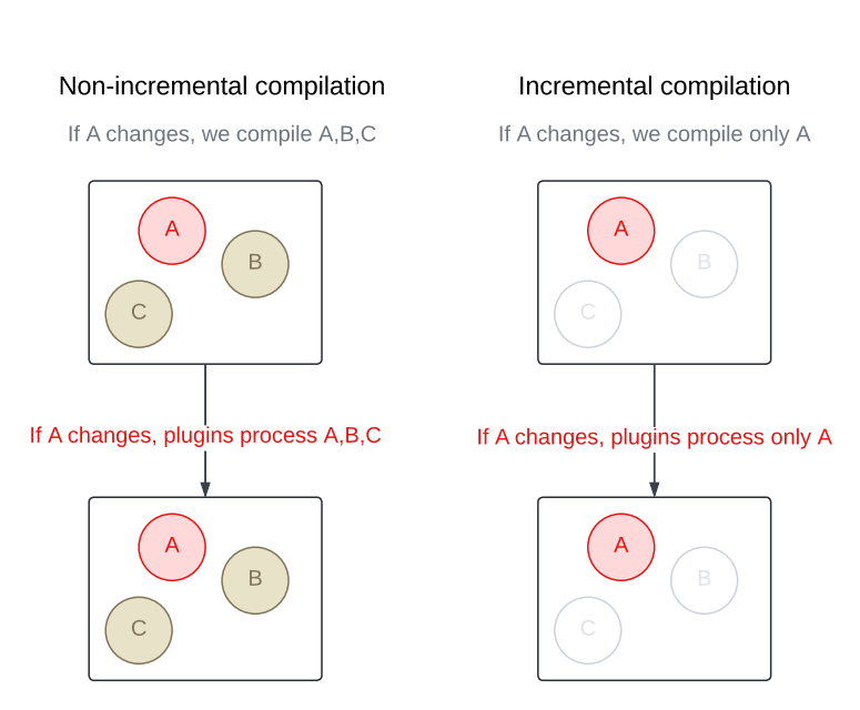
The Kotlin incremental compiler has been a true gem for developers chasing faster compilation since its introduction in build tools. Now, we’re excited to bring its benefits to Buck2 – Meta’s build system – to unlock even more speed and efficiency for Kotlin developers.
Unlike a traditional compiler that recompiles an entire module every time, an incremental compiler focuses only on what was changed. This cuts down compilation time in a big way, especially when modules contain a large number of source files.
Buck2 promotes small modules as a key strategy for achieving fast build times. Our codebase followed that principle closely, and for a long time, it worked well. With only a handful of files in each module, and Buck2’s support for fast incremental builds and parallel execution, incremental compilation didn’t seem like something we needed.
But, let’s be real: Codebases grow, teams change, and reality sometimes drifts away from the original plan. Over time, some modules started getting bigger – either from legacy or just organic growth. And while big modules were still the exception, they started having quite an impact on build times.
So we gave the Kotlin incremental compiler a closer look – and we’re glad we did. The results? Some critical modules now build up to 3x faster. That’s a big win for developer productivity and overall build happiness.
Curious about how we made it all work in Buck2? Keep reading. We’ll walk you through the steps we took to bring the Kotlin incremental compiler to life in our Android toolchain.
Step 1: Integrating Kotlin’s Build Tools API
As of Kotlin 2.2.0, the only guaranteed public contract to use the compiler is through the command-line interface (CLI). But since the CLI doesn’t support incremental compilation (at least for now), it didn’t meet our needs. Alternatively, we could integrate the Kotlin incremental compiler directly via the internal compiler’s components – APIs that are technically accessible but not intended for public use. However, relying on them would’ve made our toolchain fragile and likely to break with every Kotlin update since there’s no guarantee of backward compatibility. That didn’t seem like the right path either.
Then we came across the Build Tools API (KEEP), introduced in Kotlin 1.9.20 as the official integration point for the compiler – including support for incremental compilation. Although the API was still marked as experimental, we decided to give it a try. We knew it would eventually stabilize, and saw it as a great opportunity to get in early, provide feedback, and help shape its direction. Compared to using internal components, it offered a far more sustainable and future-proof approach to integration.
⚠️ Depending on kotlin-compiler? Watch out!
In the Java world, a shaded library is a modified version of the library where the class and package names are changed. This process – called shading – is a handy way to avoid classpath conflicts, prevent version clashes between libraries, and keeps internal details from leaking out.
Here’s quick example:
- Unshaded (original) class: com.intellij.util.io.DataExternalizer
- Shaded class: org.jetbrains.kotlin.com.intellij.util.io.DataExternalizer
The Build Tools API depends on the shaded version of the Kotlin compiler (kotlin-compiler-embeddable). But our Android toolchain was historically built with the unshaded one (kotlin-compiler). That mismatch led to java.lang.NoClassDefFoundError crashes when testing the integration because the shaded classes simply weren’t on the classpath.
Replacing the unshaded compiler across the entire Android toolchain would’ve been a big effort. So to keep moving forward, we went with a quick workaround: We unshaded the Build Tools API instead. 🙈 Using the jarjar library, we stripped the org.jetbrains.kotlin prefix from class names and rebuilt the library.
Don’t worry, once we had a working prototype and confirmed everything behaved as expected, we circled back and did it right – fully migrating our toolchain to use the shaded Kotlin compiler. That brought us back in line with the API’s expectations and gave us a more stable setup for the future.
Step 2: Keeping previous output around for the incremental compiler
To compile incrementally, the Kotlin compiler needs access to the output from the previous build. Simple enough, but Buck2 deletes that output by default before rebuilding a module.
With incremental actions, you can configure Buck2 to skip the automatic cleanup of previous outputs. This gives your build actions access to everything from the last run. The tradeoff is that it’s now up to you to figure out what’s still useful and manually clean up the rest. It’s a bit more work, but it’s exactly what we needed to make incremental compilation possible.
Step 3: Making the incremental compiler cache relocatable
At first, this might not seem like a big deal. You’re not planning to move your codebase around, so why worry about making the cache relocatable, right?
Well… that’s until you realize you’re no longer in a tiny team, and you’re definitely not the only one building the project. Suddenly, it does matter.
Buck2 supports distributed builds, which means your builds don’t have to run only on your local machine. They can be executed elsewhere, with the results sent back to you. And if your compiler cache isn’t relocatable, this setup can quickly lead to trouble – from conflicting overloads to strange ambiguity errors caused by mismatched paths in cached data.
So we made sure to configure the root project directory and the build directory explicitly in the incremental compilation settings. This keeps the compiler cache stable and reliable, no matter who runs the build or where it happens.
Step 4: Configuring the incremental compiler
In a nutshell, to decide what needs to be recompiled, the Kotlin incremental compiler looks for changes in two places:
- Files within the module being rebuilt.
- The module’s dependencies.
Once the changes are found, the compiler figures out which files in the module are affected – whether by direct edits or through updated dependencies – and recompiles only those.
To get this process rolling, the compiler needs just a little nudge to understand how much work it really has to do.
So let’s give it that nudge!
Tracking changes inside the module
When it comes to tracking changes, you’ve got two options: You can either let the compiler do its magic and detect changes automatically, or you can give it a hand by passing a list of modified files yourself. The first option is great if you don’t know which files have changed or if you just want to get something working quickly (like we did during prototyping). However, if you’re on a Kotlin version earlier than 2.1.20, you have to provide this information yourself. Automatic source change detection via the Build Tools API isn’t available prior to that. Even with newer versions, if the build tool already has the change list before compilation, it’s still worth using it to optimize the process.
This is where Buck’s incremental actions come in handy again! Not only can we preserve the output from the previous run, but we also get hash digests for every action input. By comparing those hashes with the ones from the last build, we can generate a list of changed files. From there, we pass that list to the compiler to kick off incremental compilation right away – no need for the compiler to do any change detection on its own.
Tracking changes in dependencies
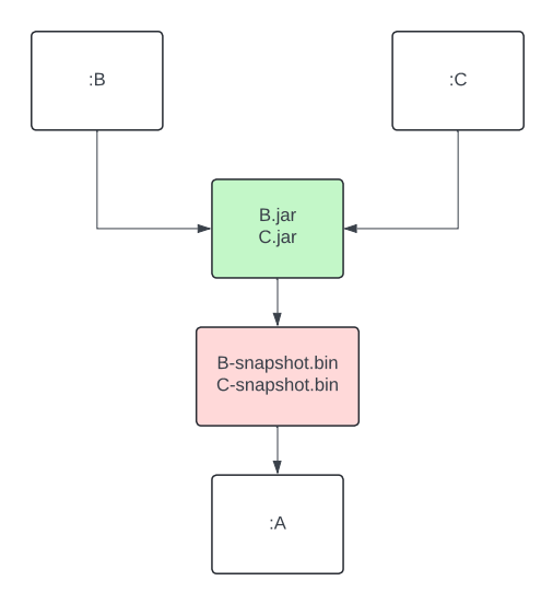
Sometimes it’s not the module itself that changes, it’s something the module depends on. In these cases, the compiler relies on classpath snapshot. These snapshots capture the Application Binary Interface (ABI) of a library. By comparing the current snapshots to the previous one, the compiler can detect changes in dependencies and figure out which files in your module are affected. This adds an extra layer of filtering on top of standard compilation avoidance.
In Buck2, we added a dedicated action to generate classpath snapshots from library outputs. This artifact is then passed as an input to the consuming module, right alongside the library’s compiled output. The best part? Since it’s a separate action, it can be run remotely or be pulled from cache, so your machine doesn’t have to do the heavy lifting of extracting ABI at this step.
If, after all, only your module changes but your dependencies do not, the API also lets you skip the snapshot comparison entirely if your build tool handles the dependency analysis on its own. Since we already had the necessary data from Buck2’s incremental actions, adding this optimization was almost free.
Step 5: Making compiler plugins work with the incremental compiler
One of the biggest challenges we faced when integrating the incremental compiler was making it play nicely with our custom compiler plugins, many of which are important to our build optimization strategy. This step was necessary for unlocking the full performance benefits of incremental compilation, but it came with two major issues we needed to solve.
🚨 Problem 1: Incomplete results
As we already know, the input to the incremental compiler does not have to include all Kotlin source files. Our plugins weren’t designed for this and ended up producing incomplete results when run on just a subset of files. We had to make them incremental as well so they could handle partial inputs correctly.
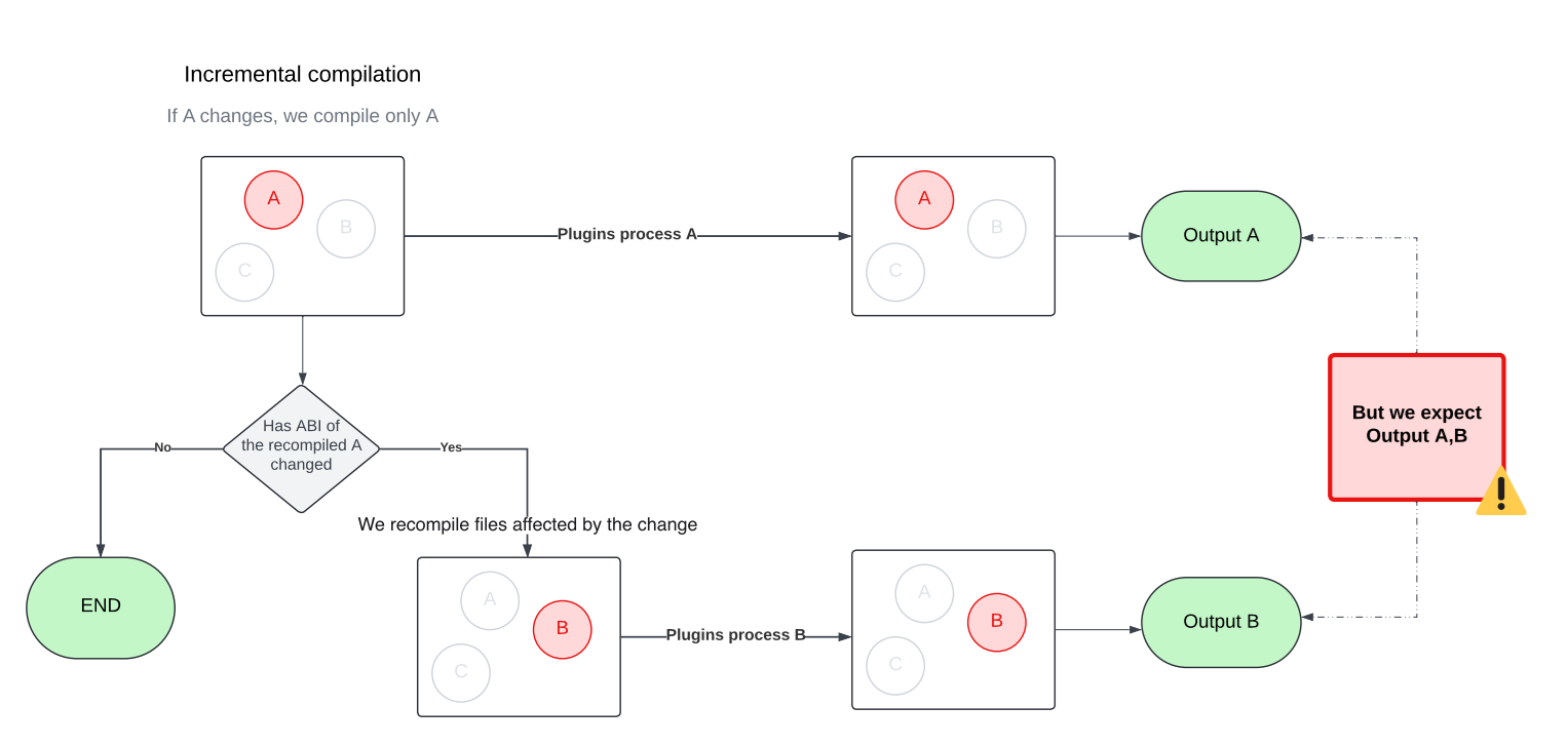
🚨 Problem 2: Multiple rounds of Compilation
The Kotlin incremental compiler doesn’t just recompile the files that changed in a module. It may also need to recompile other files in the same module that are affected by those changes. Figuring out the exact set of affected files is tricky, especially when circular dependencies come into play. To handle this, the incremental compiler approximates the affected set by compiling in multiple rounds within a single build.
💡Curious how that works under the hood? The Kotlin blog on fast compilation has a great deep dive that’s worth checking out.
This behavior comes with a side effect, though. Since the compiler may run in multiple rounds with different sets of files, compiler plugins can also be triggered multiple times, each time with a different input. That can be problematic, as later plugin runs may override outputs produced by earlier ones. To avoid this, we updated our plugins to accumulate their results across rounds rather than replacing them.
Step 6: Verifying the functionality of annotation processors
Most of our annotation processors use Kotlin Symbol Processing (KSP2), which made this step pretty smooth. KSP2 is designed as a standalone tool that uses the Kotlin Analysis API to analyze source code. Unlike compiler plugins, it runs independently from the standard compilation flow. Thanks to this setup, we were able to continue using KSP2 without any changes.
💡 Bonus: KSP2 comes with its own built-in incremental processing support. It’s fully self-contained and doesn’t depend on the incremental compiler at all.
Before we adopted KSP2 (or when we were using an older version of the Kotlin Annotation Processing Tool (KAPT), which operates as a plugin) our annotation processors ran in a separate step dedicated solely to annotation processing. That step ran before the main compilation and was always non-incremental.
Step 7: Enabling compilation against ABI
To maximize cache hits, Buck2 builds Android modules against the class ABI instead of the full JAR. For Kotlin targets, we use the jvm-abi-gen compiler plugin to generate class ABI during compilation.
But once we turned on incremental compilation, a couple of new challenges popped up:
- The jvm-abi-gen plugin currently lacks direct support for incremental compilation, which ties back to the issues we mentioned earlier with compiler plugins.
- ABI extraction now happens twice – once during compilation via jvm-abi-gen, and again when the incremental compiler creates classpath snapshots.
In theory, both problems could be solved by switching to full JAR compilation and relying on classpath snapshots to maintain cache hits. While that could work in principle, it would mean giving up some of the build optimizations we’ve already got in place – a trade-off that needs careful evaluation before making any changes.
For now, we’ve implemented a custom (yet suboptimal) solution that merges the newly generated ABI with the previous result. It gets the job done, but we’re still actively exploring better long-term alternatives.
Ideally, we’d be able to reuse the information already collected for classpath snapshot or, even better, have this kind of support built directly into the Kotlin compiler. There’s an open ticket for that: KT-62881. Fingers crossed!
Step 8: Testing
Measuring the impact of build changes is not an easy task. Benchmarking is great for getting a sense of a feature’s potential, but it doesn’t always reflect how things perform in “the real world.” Pre/post testing can help with that, but it’s tough to isolate the impact of a single change, especially when you’re not the only one pushing code.
We set up A/B testing to overcome these obstacles and measure the true impact of the Kotlin incremental compiler on Meta’s codebase with high confidence. It took a bit of extra work to keep the cache healthy across variants, but it gave us a clean, isolated view of how much difference the incremental compiler really made at scale.
We started with the largest modules – the ones we already knew were slowing builds the most. Given their size and known impact, we expected to see benefits quickly. And sure enough, we did.
The impact of incremental compilation
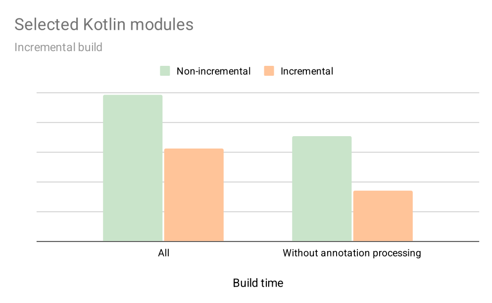
The graph below shows early results on how enabling incremental compilation for selected targets impacts their local build times during incremental builds over a 4-week period. This includes not just compilation, but also annotation processing, and a few other optimisations we’ve added along the way.
With incremental compilation, we’ve seen about a 30% improvement for the average developer. And for modules without annotation processing, the speed nearly doubled. That was more than enough to convince us that the incremental compiler is here to stay.
What’s next
Kotlin incremental compilation is now supported in Buck2, and we’re actively rolling it out across our codebase! For now, it’s available for internal use only, but we’re working on bringing it to the recently introduced open source toolchain as well.
But that’s not all! We’re also exploring ways to expand incrementality across the entire Android toolchain, including tools like Kosabi (the Kotlin counterpart to Jasabi), to deliver even faster build times and even better developer experience.
To learn more about Meta Open Source, visit our open source site, subscribe to our YouTube channel, or follow us on Facebook, Threads, X and LinkedIn.
When Andy Jassy, then head of Amazon Web Services, announced Amazon Aurora in 2014, the pitch was bold but metered: Aurora would be a relational database built for the cloud. As such, it would provide access to cost-effective, fast, and scalable computing infrastructure.
In essence, he explained, Aurora would combine the cost effectiveness and simplicity of MySQL with the speed and availability of high-end commercial databases, the kind that firms typically managed on their own. In numbers, Aurora promised five times the throughput (e.g., the number of transactions, queries, read/write operations) of MySQL at one-tenth the price of commercial database solutions, all while offloading costly management challenges and maintaining performance and availability.
AWS re:Invent 2014 | Announcing Amazon Aurora for RDS
Aurora launched a year later, in 2015. Significantly, it decoupled computation from storage, a distinct contrast to traditional database architectures where the two are entwined. This fundamental innovation, along with automated backups and replication and other improvements, enabled easy scaling for both computational tasks and storage, while meeting reliability demands.
“Aurora’s design preserves the core transactional consistency strengths of relational databases. It innovates at the storage layer to create a database built for the cloud that can support modern workloads without sacrificing performance,” explained Werner Vogels, Amazon’s CTO, in 2019.
“To start addressing the limitations of relational databases, we reconceptualized the stack by decomposing the system into its fundamental building blocks,” Vogels said. “We recognized that the caching and logging layers were ripe for innovation. We could move these layers into a purpose-built, scale-out, self-healing, multitenant, database-optimized storage service. When we began building the distributed storage system, Amazon Aurora was born.”
Within two years, Aurora became the fastest-growing service in AWS history. Tens of thousands of customers — including financial-services companies, gaming companies, healthcare providers, educational institutions, and startups — turned to Aurora to help carry their workloads.
In the intervening years, Aurora has continued to evolve to suit the needs of a changing digital landscape. Most recently, in 2024, Amazon announced Aurora DSQL. A major step forward, Aurora DSQL is a serverless approach designed for global scale and enhanced adaptability to variable workloads.
Today, International Data Corporation (IDC) research estimates that firms using Aurora see a three-year return on investment of 434 percent and an operational cost reduction of 42 percent compared to other database solutions.
But what lies behind those figures? How did Aurora become so valuable to its users? To understand that, it’s useful to consider what came before.
A time for reinvention
In 2015, as cloud computing was gaining popularity, legacy firms began migrating workloads away from on-premises data centers to save money on capital investments and in-house maintenance. At the same time, mobile and web app startups were calling for remote, highly reliable databases that could scale in an instant. The theme was clear: computing and storage needed to be elastic and reliable. The reality was that, at the time, most databases simply hadn’t adapted to those needs.
Amazon engineers recognized that the cloud could enable virtually unlimited, networked storage and, separately, compute.
That rigidity makes sense considering the origin of databases and the problems they were invented to solve. The 1960s saw one of their earliest uses: NASA engineers had to navigate a complex list of parts, components, and systems as they built spacecraft for moon exploration. That need inspired the creation of the Information Management System, or IMS, a hierarchically structured solution that allowed engineers to more easily locate relevant information, such as the sizes or compatibilities of various parts and components. While IMS was a boon at the time, it was also limited. Finding parts meant engineers had to write batches of specially coded queries that would then move through a tree-like data structure, a relatively slow and specialized process.
In 1970, the idea of relational databases made its public debut when E. F. Codd coined the term. Relational databases organized data according to how it was related: customers and their purchases, for instance, or students in a class. Relational databases meant faster search, since data was stored in structured tables, and queries didn’t require special coding knowledge. With programming languages like SQL, relational databases became a dominant model for storing and retrieving structured data.
By the 1990s, however, that approach began to show its limits. Firms that needed more computing capabilities typically had to buy and physically install more on-premises servers. They also needed specialists to manage new capabilities, such as the influx of transactional workloads — as, for instance, when increasing numbers of customers added more and more pet supplies to virtual shopping carts. By the time AWS arrived in 2006, these legacy databases were the most brittle, least elastic component of a company’s IT stack.
The emergence of cloud computing promised a better way forward with more flexibility and remotely managed solutions. Amazon engineers recognized that the cloud could enable virtually unlimited, networked storage and, separately, computation.
The Amazon Relational Database Service (Amazon RDS) debuted in 2009 to help customers set up, operate, and scale a MySQL database in the cloud. And while that service expanded to include Oracle, SQL Server, and PostgreSQL, as Jeff Barr noted in a 2014 blog post, those database engines “were designed to function in a constrained and somewhat simplistic hardware environment.”
AWS researchers challenged themselves to examine those constraints and “quickly realized that they had a unique opportunity to create an efficient, integrated design that encompassed the storage, network, compute, system software, and database software”.
“The central constraint in high-throughput data processing has moved from compute and storage to the network,” wrote the authors of a SIGMOD 2017 paper describing Aurora’s architecture. Aurora researchers addressed that constraint via “a novel, service-oriented architecture”, one that offered significant advantages over traditional approaches. These included “building storage as an independent fault-tolerant and self-healing service across multiple data centers … protecting databases from performance variance and transient or permanent failures at either the networking or storage tiers.”’
The serverless era is now
In the years since its debut, Amazon engineers and researchers have ensured Aurora has kept pace with customer needs. In 2018, Aurora Serverless provided an on-demand autoscaling configuration that allowed customers to adjust computational capacity up and down based on their needs. Later versions further optimized that process by automatically scaling based on customer needs. That approach relieves the customer of the need to explicitly manage database capacity; customers need to specify only minimum and maximum levels.
Achieving that sort of “resource elasticity at high levels of efficiency” meant Aurora Serverless had to address several challenges, wrote the authors of a VLDB 2024 paper. “These included policy issues such as how to define ‘heat’ (i.e., resource usage features on which to base decision making)” and how to determine whether remedial action may be required. Aurora Serverless meets those challenges, the authors noted, by adapting and modifying “well-established ideas related to resource oversubscription; reactive control informed by recent measurements; distributed and hierarchical decision making; and innovations in the DB engine, OS, and hypervisor for efficiency.”
As of May 2025, all of Aurora’s offerings are now serverless. Customers no longer need to choose a specific server type or size or worry about the underlying hardware or operating system, patching, or backups; all that is completely managed by AWS. “One of the things that we’ve tried to design from the beginning is a database where you don’t have to worry about the internals,” Marc Brooker, AWS vice president and Distinguished Engineer, said at AWS re:Invent in 2024.
These are exactly the capabilities that Arizona State University needs, says John Rome, deputy chief information officer at ASU. Each fall, the university’s data needs explode when classes for its more than 73,000 students are in session across multiple campuses. Aurora lets ASU pay for the computation and storage it uses and helps it to adapt on the fly.
We see Amazon Aurora Serverless as a next step in our cloud maturity.
John Rome, deputy chief information officer at ASU
“We see Amazon Aurora Serverless as a next step in our cloud maturity,” Rome says, “to help us improve development agility while reducing costs on infrequently used systems, to further optimize our overall infrastructure operations.”
And what might the next step in maturity look like for the now 10-year-old Aurora service? The authors of that 2024 paper outlined several potential paths. Those include “introducing predictive techniques for live migration”; “exploiting statistical multiplexing opportunities stemming from complementary resource needs”, and “using sophisticated ML/RL-based techniques for workload prediction and decision making.”
-
Tools & Platforms3 weeks ago
Building Trust in Military AI Starts with Opening the Black Box – War on the Rocks
-

 Business3 days ago
The Guardian view on Trump and the Fed: independence is no substitute for accountability | Editorial
-

 Ethics & Policy1 month ago
SDAIA Supports Saudi Arabia’s Leadership in Shaping Global AI Ethics, Policy, and Research – وكالة الأنباء السعودية
-

 Events & Conferences3 months ago
Journey to 1000 models: Scaling Instagram’s recommendation system
-

 Jobs & Careers2 months ago
Mumbai-based Perplexity Alternative Has 60k+ Users Without Funding
-

 Funding & Business2 months ago
Kayak and Expedia race to build AI travel agents that turn social posts into itineraries
-

 Education2 months ago
VEX Robotics launches AI-powered classroom robotics system
-

 Podcasts & Talks2 months ago
Happy 4th of July! 🎆 Made with Veo 3 in Gemini
-

 Podcasts & Talks2 months ago
OpenAI 🤝 @teamganassi
-

 Mergers & Acquisitions2 months ago
Donald Trump suggests US government review subsidies to Elon Musk’s companies