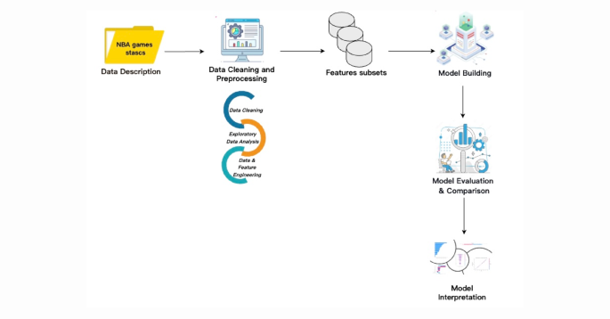
This study aims to develop a predictive framework for NBA game outcomes using a machine-learning strategy based on the Stacking ensemble method. This section details the materials and methods used to achieve our objective. Figure 1 displays the overall workflow of the proposed framework. The entire experimental procedure was carried out in a Jupyter Notebook environment using Python. We utilized several key Python libraries—including NumPy, Pandas, Scikit-learn, and Matplotlib—for data processing, model development, and result visualization.

Dataset

The data used in this study were obtained from the official NBA website (https://www.nba.com), which provides a comprehensive collection of multi-dimensional information, including basic player and team statistics, advanced efficiency metrics, spatial tracking data, lineup performance, and salary and management records. These datasets are widely used in both tactical analysis and machine learning modeling.

This study focuses primarily on game-level performance and outcomes from the regular seasons of the 2021–2022, 2022–2023, and 2023–2024 NBA seasons. Specifically, data were collected from all 1,230 games per season, totaling 3,690 games and 7,380 samples (accounting for both home and away teams). The dataset comprises 20 feature variables, including total field goals made, three-point shots made, and other offensive and defensive indicators. The game outcome (win or loss) serves as the target variable. Detailed descriptions of all variables are provided in Table 2.

Data processing

To facilitate model training, the game outcome variable for all regular-season games across the three NBA seasons was encoded as a binary classification variable, where a win was labeled as 1 and a loss as 0. This binary encoding allows machine learning models to distinguish between game outcomes more effectively.

As shown in the summary statistics presented in Table 3, the resulting dataset is balanced, containing an equal number of win and loss samples. Specifically, among the 7,380 total samples, there are 3,690 observations for each class (win and loss).

Dataset partitioning

To prevent model overfitting and ensure robust predictive performance, the dataset was randomly partitioned into training and testing subsets. Given that each regular-season game across the three NBA seasons is mutually independent, random sampling was employed for the split.

Specifically, 80% of the data was allocated to the training set, and the remaining 20% to the testing set. The training set was used for model construction, while the testing set was used for evaluating the model’s performance. The detailed distribution of samples is presented in Table 4.

Feature selection

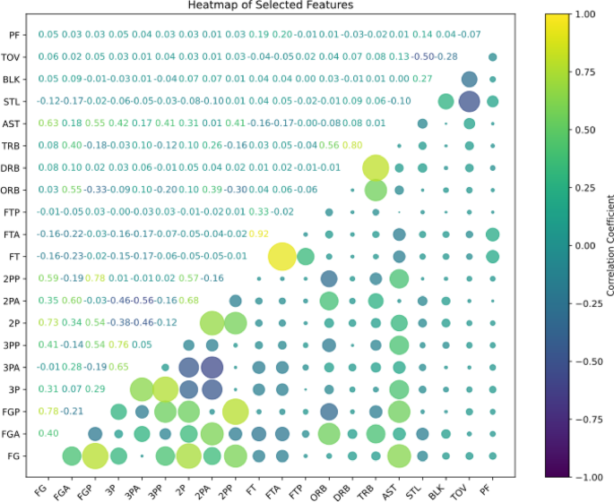
Feature selection is a crucial step that directly impacts the accuracy and generalization performance of a model²⁰. To prevent the issue of multicollinearity among variables, which can reduce model interpretability, key features were further screened to address this concern. We employed Exploratory Data Analysis (EDA) techniques and calculated the Pearson correlation coefficients between feature variables to assess inter-variable relationships visually. As shown in the correlation heatmap in Fig. 2, no severe multicollinearity was observed among the 20 feature variables. Therefore, all 20 features were retained for model training and analysis. Descriptive statistics for each variable are presented in Table 5.

Pearson Correlation Heatmap of Feature Variables.

Model building

After completing data preprocessing, this study utilizes the Scikit-Learn Python toolkit to train machine learning models. The dataset is initially divided into training and testing sets, ensuring a systematic approach to model evaluation. Various machine learning classifiers are then applied to train and evaluate the model’s performance, allowing for a thorough comparison of their predictive abilities.

To construct the baseline models, each candidate machine learning algorithm is evaluated using 5-fold cross-validation, a widely accepted technique to ensure robust and unbiased performance estimation. The model yielding the highest average accuracy across folds is selected for inclusion in the base layer of the Stacking ensemble framework. The accuracy metric computed via 5-fold cross-validation is formally defined in Eq. 1.

In this context, k represents the number of cross-validation folds, while Ai indicates the accuracy achieved on the i-th fold. The resulting CA_k represents the model’s average cross-validated accuracy. According to the evaluation results above, the models with the highest accuracy are selected to form the base layer of the Stacked Ensemble. The selection criterion is further specified in Eq. 2.

Let modeli represent the selected model, while O (max…min) indicates the descending order function based on the cross-validation accuracies of n different models. The top-performing models are chosen to form the foundation of the proposed Stacked Ensemble Model.

Selected models

Multilayer perceptron

The Single-Layer Perceptron is limited in its ability to solve problems that are not linearly separable. The MLP was developed as an extension to address this limitation. The MLP incorporates a multilayer network architecture trained using the backpropagation algorithm. The architecture generally includes three-layer types: the input layer, one or more hidden layers, and the output layer²¹. In contrast to the Single-Layer Perceptron, the MLP includes at least one intermediate (hidden) layer that enables the model to capture non-linear relationships²².

XGBoost

XGBoost is an ensemble learning algorithm that generates predictions by aggregating the outputs of multiple base learners, typically decision trees²³. While it shares structural similarities with Random Forest in using decision trees as fundamental components, XGBoost offers notable advantages over traditional Gradient Boosting Decision Tree (GBDT) methods. These include significantly faster computational speed, improved generalization performance, and superior scalability, making it well-suited for large-scale and high-dimensional machine learning tasks. Unlike many machine learning frameworks, XGBoost offers extensive support for fine-tuning regularization parameters, providing greater control over model complexity and improving overall performance²⁴. Due to its efficiency and strong generalization capability, XGBoost has become a widely used technique for predictive modeling across various domains, including sports analytics and NBA game outcome prediction.

AdaBoost

AdaBoost is an ensemble learning method that builds a strong classifier by iteratively combining multiple weak learners. In each iteration, more focus is placed on instances that were misclassified in the previous round, guiding subsequent classifiers to concentrate on more challenging samples. AdaBoost classifiers operate as meta-estimators, initially training a base learner on the original dataset²⁵. In the following iterations, the same base learner is retrained multiple times but with adjusted sample weights—specifically, increasing the weights of previously misclassified instances—so that the model progressively improves its performance on complex examples.

Naive Bayes

This classification algorithm, named after the English mathematician Thomas Bayes, is based on Bayes’ theorem, and relies on probabilistic reasoning. It performs classification by applying probability calculations derived from training data and assigns a new instance to the class with the highest posterior probability²⁴. The mathematical formulation of Bayes’ theorem is presented in Eq. 3.

P (A | B) represents the probability of event A occurring, given that event B has already occurred.

P (B | A) denotes the likelihood of event B occurring, given that event A has occurred.

P(A) and P(B) refer to the prior (unconditional) probabilities for events A and B, respectively.

K-Nearest neighbor (KNN)

The K-nearest neighbor (KNN) algorithm is a supervised learning technique used for both classification and regression tasks. It is a non-parametric, instance-based learning algorithm that makes predictions based on the similarity between data points. In the classification process, when a new sample needs to be categorized, the algorithm identifies the k closest data points from the training set based on a chosen distance metric (e.g., Euclidean distance, Manhattan distance, or Minkowski distance). The majority class among these K nearest neighbors is then assigned as the class label for the new sample²⁶.

Logistic regression

Logistic Regression is a regression-based classification method primarily designed for binary classification problems. It can be considered an extension of Linear Regression, optimized to estimate the probability that a given observation belongs to a particular category. In other words, Logistic Regression predicts the likelihood of an outcome based on a set of independent variables and then classifies the dependent variable accordingly²⁶.

Decision tree

A Decision Tree is a supervised learning model for classification and regression tasks. It follows a hierarchical, tree-like structure to recursively partition the dataset based on feature values, ultimately reaching a leaf node representing the predicted outcome^27,28.

Proposed stacked ensemble model

This study proposes a Stacked Ensemble (Stacking) model to enhance overall performance by integrating predictions from multiple base models. Stacking enables the training of diverse machine learning models to solve similar problems, combining their outputs to construct a more robust and accurate predictive model^28,29. In contrast to ensemble techniques like Bagging and Boosting, Stacking emphasizes the integration of heterogeneous and strong base models, utilizing their complementary capabilities to enhance overall predictive performance. By aggregating the predictions of multiple models, the approach enhances generalization ability and performance stability.

The Stacking ensemble framework can be formally defined as follows: Given a k-fold cross-validation setup, let (x, y)k represent the k data folds, x = (x₁, x₂, …, xr) corresponds to the r recorded feature values, and y = (x_r+1, x_r+2, …, x_r+p) represents the p target values to be predicted. For a given set of N potential learning algorithms, denoted as modeli, i = 1, …, N, Let A_ij represent the model created by algorithm modeli trained on x to predict x_p+j. The generalizer function, denoted as G_j, is responsible for merging predictions from the base models to produce the final forecast. G_j can be either a meta-model trained via a learning algorithm or a general function such as a weighted average. Thus, the estimated prediction value \(\hat{x}\) (p + j) can be formally expressed by Eq. 4. The training process is shown in Fig. 3. The effectiveness of the Stacking ensemble learning method relies on two key factors: (1) the performance of the base classifiers—the better the performance of the base models, the higher the overall ensemble performance; and (2) the diversity among the base classifiers. Introducing heterogeneous base models allows each to contribute uniquely, improving the ensemble model’s generalization capability.

Training Process of the Stacking Ensemble Learning Model.

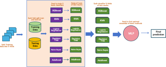
In this study, the stacked ensemble method was constructed by selecting six classifiers—XGBoost, KNN, AdaBoost, Naive Bayes, Logistic Regression, and Decision Tree—from multiple candidate models based on their highest cross-validation accuracy, which served as the base layer of the ensemble model. At the second layer, a MLP was used as the meta-learner (super learner). The MLP consisted of two hidden layers, each comprising 50 neurons, and was responsible for aggregating the prediction outputs from the base classifiers to produce the final prediction.

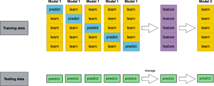
The complete training process is illustrated in Fig. 4 and follows a 5-fold cross-validation scheme. Specifically, the training data were randomly divided into five equally sized folds. In each iteration, four folds were used for training and the remaining fold served as the validation set. This process was repeated five times, ensuring that each fold functioned as the validation set once. During each fold, all six base classifiers were trained on the training subset and used to generate predictions on the corresponding validation fold. This resulted in five prediction sets per classifier. These out-of-fold predictions were then concatenated to form a new feature matrix, which served as the input to the meta-learner for training.

Simultaneously, predictions were made on the test set in each fold using the base classifiers, and the average of these predictions was used to construct the test set input for the meta-learner. Finally, the MLP meta-classifier used these new features to produce the final prediction results.

Complete the Training Process of the Stacking Model with 5-Fold Cross-Validation.

Interpretability analysis

The model’s predictions are analyzed using SHAP (Shapley Additive Explanations) values, which measure the contribution of each feature to the output for a specific instance. SHAP is grounded in cooperative game theory, where the model prediction is treated as a total reward, and the feature values are considered players contributing to this reward³⁰.

Consider a dataset that contains p features, represented by the set F = {1, 2, 3, …, p}. A subset of features C ≤ F is referred to as a coalition, representing a collective contribution to the prediction. The empty set, denoted as \(\:\tau\:\), represents a scenario with no contributing features. A characteristic function v is defined to assign a real value to each subset C, such that v(C) reflects the predictive value of the coalition. To determine the individual contribution of feature i, SHAP evaluates all possible permutations of the feature set and computes the average marginal contribution of feature i across all coalitions that exclude i. The SHAP value \(\:\tau\:\)_i for feature i is formally defined in Eq. 5.

We utilize SHAP (Shapley Additive Explanations) analysis to enhance the interpretability of our NBA game prediction model. Specifically, we apply Kernel SHAP to perform both Global Mean Analysis and Local Interpretability, enabling us to quantify the influence of individual features on the model’s predictions across different scenarios.

Global interpretability

Global interpretability assesses how individual features influence the model’s predictions on average. The horizontal axis represents the average change in model output when a specific feature is omitted or “masked.” In this context, “masked” signifies that the feature is removed from the input, thereby eliminating its influence on the prediction. Let N denote the total number of samples, \(\:{\varphi\:}_{i}^{\left(j\right)}\) represent the SHAP value of the i-th feature for the j-th sample, and \(\:{\varPhi\:}_{i}^{global}\)denote the global average SHAP importance of the i-th feature. The Global SHAP value can be represented using Eq. 6 as follows:

Local interpretability

Local interpretability explains individual predictions, analyzing key factors driving specific NBA game outcomes. Where f(x): the model’s prediction output for sample x; ∅₀ the model’s baseline output (typically the expected output over background data); ∅_i the SHAP value of feature i for the given sample, representing the individual contribution of feature i to the prediction; p the total number of features. The Local SHAP Approximation Model can be represented using Eq. 7 as follows:

Performance matrix

This study applies multiple machine learning models, with their effectiveness evaluated through performance metrics: Accuracy, Precision, Recall, and F1-score, each formally described in Eqs. 8, 9, 10, and 11³¹. In this context, TP, FP, TN, and FN represent True Positives, False Positives, True Negatives, and False Negatives, respectively. In addition to these conventional metrics, the Receiver Operating Characteristic – Area Under the Curve (ROC-AUC) is used to evaluate classification quality. The ROC curve depicts the relationship between the True Positive Rate (TPR), which is the same as Recall, and the False Positive Rate (FPR) as defined in Eqs. 9 and 12. This curve offers a comprehensive visualization of a model’s diagnostic ability across all possible classification thresholds, allowing for an assessment of its overall discriminative power.