AI Research
Type II mechanoreceptors and cuneate spiking neuronal network enable touch localization on a large-area e-skin

Sensitive FBG-based e-skin
The experimented e-skin (Extended Data Fig. 5) had size and shape similar to those of the human forearm. To mimic biomechanical compliance, a soft silicone polymer (Dragon Skin 10 medium, Smooth-On) was used to realize a flexible patch to embed an optical fibre with 21 FBG sensors. It was fabricated by a three-step process11: (1) a first silicone pouring in a custom mould to obtain a bottom layer with a groove; (2) the embedding of the fibre along the grooved path; (3) a second silicone pouring to cover the fibre itself and provide robustness to the patch. The e-skin was then attached to a custom three-dimensionally printed plastic support to guarantee stability. The optically sensitive elements were FBGs (length, 10 mm) distributed along the designed path running throughout the e-skin resemble the sensitivity features of the human forearm, that is, with an increasing density from the proximal to distal parts. These gratings are interference patterns inscribed within the core of a single optical fibre. When broadband spectrum light, sent by means of an optoelectronic interrogator, passes through the fibre cable and hits an FBG, it is partly back-reflected to the input point, as a spectral peak centred at a characteristic wavelength, λB:
$${\lambda }_{\rm{B}}=2 {n}_{{{\rm{eff}}}}\varLambda,$$
(1)
where neff is the effective refractive index of the optical fibre and Λ is the pitch of the specific grating80. The λB value of the e-skin FBGs were, hence, defined by fabrication and ranged between 1,520 nm and 1,580 nm with a step of 3 nm. Wavelength shifts occur when a deformation is applied to the sensor11, thereby allowing the encoding of tactile stimuli. Considering this feature and to reduce the effects of potential prestrains that could have impacted the residual deformability of the sensors in response to external tactile stimuli, the FBGs were arranged on straight fibre segments.
Indentation data collection
The training and validation of the proposed model required the collection of a dataset of indentations applied over the e-skin surface. For this purpose, an automatized indentation protocol was executed, with 1,846 target points to touch, computed as the centroids of the triangles of a random mesh of the skin surface. A bimanual robotic platform, consisting of two anthropomorphic arms (Racer-5-0.80, Comau), was programmed to cooperate during the indentation protocol (Extended Data Fig. 5): one robot performed the tactile tasks, whereas the other held and oriented the e-skin. The indenting robot reached each target site perpendicularly, touching the skin with a spring-like hemispherical probe attached to the end-effector. Force feedback measured by means of a load cell (Nano 43, ATI Industrial Automation), mounted at the base of the indenter, was provided to control the robot to release the contact when exceeding a threshold (2.5 N) and then fly to a new target point. The control code consisted of dedicated routines (LabVIEW, National Instruments) running on both an industrial controller (IC-3173, National Instruments), to send commands to the robots, and a PC, for managing and checking the experiments. During the indentation sessions, force and FBG signals, the latter read by means of an optical interrogator (FBG Scan 904, FBGS Technologies), were collected at a 100-Hz rate, and saved into text files together with the Cartesian coordinates of the contact sites.
Assessment of receptive fields of e-skin FBG sensors
The receptive fields of the FBG sensors populating the skin were represented as two-dimensional contour maps depicting the spatial distribution of sensitivity to contact force. Hotspot regions in dark blue indicate the maximum sensitivity (Fig. 1b and Extended Data Fig. 1). To obtain the FBG receptive fields, the wavelength variation signals (Δλ) from each FBG sensor were averaged over 500 ms captured on the highest force plateau, that is, the second force level, and divided by its average value. The obtained results were then normalized with respect to the highest FBG sensitivity value, to have sensitivity maps ranging from 0 to 1. This procedure was performed using all the available indentation samples.
First-order neurons: type II PA model
The 21 FBG signals were the input of the PA models. Each sensor signal was resampled at a frequency of 1 kHz to establish a regular firing dynamics consistent with the discretization of the Izhikevich neuronal model74. The FBG signal derivatives were computed to obtain the dynamic components of the indentations, that is, the loading and unloading phases of the varying force levels applied to the e-skin. The absolute values of both raw and differentiated signals were calculated to feed the Izhikevich neurons as input current I, to mimic the adaptation dynamics and firing response of type II mechanoreceptors, that is, Ruffini endings (SAII) and Pacini corpuscles (FAII)38. To simulate the physiology of type II PAs in terms of the ratio between slowly and fast-adapting units, that is, two SAIIs to one FAII36, their diverse sensitivity and the different-sized overlapping receptive fields, the raw absolute FBG signals and their derivatives were multiplied by four and two distinct gains. Hence, six mechanoreceptor models were considered for each FBG sensor (Fig. 2), resulting in 126 input currents for the first-order neuron models. Extended Data Table 1 shows the gains used for the SAII and FAII models. The SAII gains were selected through some pilot tests and empirical analyses, where we assessed whether the increase in gain was generating an increase in the firing rate within the physiological range documented in the literature43. Specifically, the average ISIs (that is, the inverse of the average firing rates) corresponding to each force range were computed, and their logarithmic values were fitted to the logarithm of the stimulus intensity percentage (force values normalized by the maximum of 4 N; Fig. 2h). The results were then compared with background neurophysiological findings43, particularly to the ISI characterization of SAII units. The FAII gains were selected following the same empirical approach, that is, by evaluating the spiking activity at load transients. It is worth noticing that a general procedure for establishing the gains of the input currents of the Izhikevich model for artificial mechanoreceptor simulation has not yet been established in the literature. Thus, several studies, such as ref. 58, reported this empirical method of gain selection according to the specific application.
The Izhikevich model consists of a system of differential equations that can be solved via the Euler method74. Equation (2) describes the dynamics of the membrane potential v of the neuron; equation (3) represents the recovery variable u, responsible for the repolarization of the neural membrane; equation (4) describes the membrane potential restoration and the recovery variable update when v reaches the 30-mV firing threshold:
$$\frac{{{\rm{d}}v}}{{{\rm{d}}t}}=A{v}^{2}+{Bv}+C-u+{{{\rm{Gain}}}}_{n}\frac{I\left(t\right)}{{C}_{{\rm{m}}}},$$
(2)
$$\frac{{{\rm{d}}u}}{{{\rm{d}}t}}=a\left({bv}-u\right),$$
(3)
$${\rm{If}}\,v\ge 30\,{{\rm{mV}}},{\rm{then}}\left\{\begin{array}{c}v\leftarrow c\\ u\leftarrow u+d\end{array}\right.,$$
(4)
where A, B, and C are standard variables of the Izhikevich model; t represents time; a is the timescale of u; b is the sensitivity of u to the membrane potential; c is the membrane resting potential value; and d modulates the dynamics of the after-spike reset of the recovery variable u. For the implemented mechanoreceptors, we choose the parameters Gainn (Extended Data Table 1) that reproduced a regular firing behaviour.
Encoding of contact intensity by SNN PAs
The activity of type II mechanoreceptors was analysed to investigate relationships with the intensity of the applied load. For this purpose, the perpendicular force profile was extracted for all the 1,846 indentations. For each indentation, SAII and FAII units were considered separately. First, their corresponding firing rates were calculated on moving time windows of 100 ms, with an overlap of 50 ms. For each window, the firing rate was extracted as follows:
$${{{\rm{FR}}}}_{X}=\frac{{N}_{{{\rm{spikesX}}}}}{{w}_{{{{\rm{t}}}}} {N}_{{{\rm{neuronXactive}}}}},$$
where the subscript X indicates the type of mechanoreceptor (SAII or FAII), wt is the duration of the time window, NspikesX is the number of spikes of the X units in wt and NneuronXactive is the number of active neurons of each type in the selected window. The resulting firing rates were compared with the corresponding force profile (Fig. 2a–f). Then, the SAII firing rates were grouped for force levels, ranging from 0 to 4 N, with a step of 0.5 N. The corresponding distributions were analysed and the relevant statistics computed (median values and first and third quartiles; Fig. 2g and Supplementary Table 1). For each load-intensity level, the mean SAII firing rate value was extracted to further derive the relationship with the applied loads. For that, the linear Pearson correlation coefficient ρ was calculated. Then, the first-order polynomial that fitted the logarithm of the SAII average firing rates to the logarithm of the percentage of the applied load, normalized by 4 N, was extrapolated. The R2 coefficient was computed to assess the goodness of the linear fit (Fig. 2h).
Second-order neurons: CN model
The second layer of the SNN was composed of 1,036 CNs, modelled with the mathematical implementation based on the exponential integrate-and-fire approach29. This model reproduces the complete dynamics of the membrane potential of CNs, as described in equation (5), along with a detailed modelling of the activity of low-threshold voltage-gated calcium channels and calcium-activated potassium channels:
$${C}_{{\rm{m}}}\frac{{{{\rm{d}}V}}_{{\rm{m}}}}{{{\rm{d}}t}}={I}_{{\rm{L}}}+{I}_{{{\rm{spike}}}}+{I}_{{{\rm{ion}}}}+{I}_{{{\rm{ext}}}}+{I}_{{{\rm{syn}}}}.$$
(5)
In equation (5), Cm is the capacitance of the neural membrane; Vm is the CN membrane potential; IL is the leak current of the neuron (equation (6)); Ispike is the spike current that recreates the action potential onset and the fast neuron depolarization (equation (7)); Iion is the ionic current resulting from the summation of the currents of voltage-gated calcium channels (ICa) and calcium-activated potassium channels (IK; equation (8)); Iext is the external current that can be injected into the neuron (in this study, it is equal to 0); and Isyn is the synaptic current (equation (9)), where each synapse (i) is activated by a PA.
$${I}_{{\rm{L}}}={-\bar{g}}_{{\rm{L}}}\left({V}_{{\rm{m}}}-{E}_{{\rm{L}}}\right),$$
(6)
$${I}_{{{\rm{spike}}}}={\bar{g}}_{{\rm{L}}{\rm{L}}}{\Delta}_{{\rm{t}}}\exp \left(\frac{{V}_{{\rm{m}}}-{V}_{{\rm{t}}}}{{\Delta }_{{\rm{t}}}}\right),$$
(7)
$${I}_{{{\rm{ion}}}}={I}_{{{\rm{Ca}}}}+{I}_{{\rm{K}}},$$
(8)
$$\begin{array}{l}{I}_{{{\rm{syn}}}}={g}_{\max }\sum _{i}{w}_{{{\rm{exc}}},i}\exp \left(-\tau \left(t-{t}^{* }\right)\right)\left({E}_{{{\rm{rev}}},{{\rm{exc}}}}-{V}_{{\rm{m}}}\right)\\\qquad\;\;+\,{g}_{\max }{w}_{{{\rm{inh}}}}\sum _{i}\exp \left(-\tau \left(t-{t}^{* }\right)\right)\left({E}_{{{\rm{rev}}},{{\rm{inh}}}}-{V}_{{\rm{m}}}\right),\end{array}$$
(9)
where wexc,i is the excitatory synaptic weight; t* is the time at which a spike occurs and winh is the inhibitory synaptic weight. Isyn can be, hence, expressed as the sum of the excitatory and inhibitory synaptic currents of all the synapses of the individual PAs. The definitions of the other variables and their respective values are reported in Supplementary Table 6.
The current ICa is described by equation (10) and the current IK, by equation (11):
$${I}_{{{\rm{Ca}}}}=-{\bar{g}}_{{{\rm{Ca}}}}{x}_{{{\rm{Ca}}},{a}}^{3}{x}_{{{\rm{Ca}}},i}\left({V}_{{\rm{m}}}-{E}_{{{\rm{Ca}}}}\right),$$
(10)
$${I}_{{\rm{K}}}=-{\bar{g}}_{{\rm{K}}}{x}_{{{\rm{K}}}_{{{\rm{Ca}}}}}^{4}{x}_{{{\rm{K}}}_{{{\rm{V}}_{\rm{m}},}}}^{4}\left({V}_{{\rm{m}}}-{E}_{{\rm{K}}}\right),$$
(11)
where \({\bar{g}}_{{{\rm{Ca}}}}\) and \({\bar{g}}_{{\rm{K}}}\) are the maximum conductance; ECa and EK are the action potentials of the calcium and potassium channels, respectively; and xCa,a, xCa,i, \({x}_{{{\rm{K}}}_{{{\rm{Ca}}}}}\) and \({x}_{{{\rm{K}}}_{{{\rm{V}}_{\rm{m}}}}}\) are the activity states of the channels. These values are provided in Supplementary Table 6.
In this model, both ion channels (xCa,a and xCa,i) are considered as sources of the membrane calcium concentration of the CN ([Ca2+]). Thus, we proposed that the activity of the total neuron calcium concentration follows equation (12).
$$\begin{array}{l}\frac{{\rm{d}}\left(\left[{{{\rm{Ca}}}}^{2+}\right]\right)}{{{\rm{d}}t}}={{\rm{BCa}}}\bar{g}{C}_{a}{x}_{{{\rm{Ca}}}{,a}}^{3}x{C}_{a,i}\left({V}_{{\rm{m}}}-{E}_{{{\rm{Ca}}}}\right)\\\qquad\qquad\;+\,\left(\left[{{{\rm{Ca}}}}^{2+}\right]_{{{\rm{rest}}}}-\left[{{{\rm{Ca}}}}^{2+}\right]\right)/{\tau }_{\left[{{{\rm{Ca}}}}^{2+}\right]}.\end{array}$$
(12)
The relevant parameters are reported in Supplementary Table 2.
Functional organization of SNN second-order neurons to model a somatotopic map of the e-skin
To functionally mimic the organization of the cuneate nucleus, we generated an e-skin grid mesh with 29 × 38 edges, that is, 28 × 37 subregions. In this mesh, each subregion represented a CN, and its centroid represented the centre of its receptive field. In total, 1,036 CNs were created with circular overlapping receptive fields of 41.67-mm radius each. The criterion for the definition of the size of the CN receptive field was to include at least two FBG sensors in the corresponding sensitive area of the e-skin and, thus, 12 PAs, consistent with the number of dominant PAs that project into a CN found in neurophysiological studies on mammals and simulations of human tactile perception24. This approach allowed us to determine a CN somatotopic map of the e-skin.
Connectivity of SNN and initialization of synaptic weights
In our model, each of the 1,036 CNs was fully connected to the 126 PAs, with excitatory weights ranging from 0 to 1, and to a single inhibitory synapse (Fig. 1a, red triangle), with an IN that grouped the responses of all the 126 PA projections (Fig. 1a, coloured empty triangles). This connectivity enabled the potentiation or depression of all the synaptic weights during the learning process. In this model, the magnitude of the postsynaptic potential projected into a CN for a given sensory input is dependent on both excitatory (wexc,i) and inhibitory (winh) weights, as described in equation (9)18,29. The presynaptic excitatory weights were initialized as the inverse of the Euclidean distances between the position of the 21 FBG sensors in the skin and the 1,036 centroids of the CNs. Then, the obtained values were rescaled between 0.2 and 1. The initial excitatory weights (wexc) of the PAs corresponding to the sensors outside the area of the CN receptive fields were instead set to 0 (Fig. 1a, coloured dots). In this way, only the mechanoreceptors inside the CN receptive field region had initial weights greater than 0 (Fig. 1a, coloured filled triangles). All the inhibitory synaptic weights (winh) were instead initialized to 0.125.
Synaptic learning protocol of SNN second-order neurons
Inspired by calcium-dependent synaptic plasticity, we implemented a synaptic learning process29, where the total inhibitory weights (winh) and presynaptic excitatory weights (wexc,i) were updated at each stimulus presentation. According to our model, the excitatory weight potentiation of the presynaptic neurons (PAs) occurred when the total calcium activity (\({A}_{{{\rm{Tot}}}}^{{{{\rm{Ca}}}}^{2+}}\)) of the CN, as in equation (13), was strongly correlated with the local calcium activity (\({A}_{{{\rm{Loc}}}_{i}}^{{{{\rm{Ca}}}}^{2+}}\)) of a synapse (PA with the secondary neuron; equation (14)); otherwise, this synapse was depressed:
$${A}_{\rm{Tot}}^{{\rm{Ca}}^{2+}}={k}_{{{\rm{act}}}} \times [{{\rm{Ca}}}^{2+}],$$
(13)
$${A}_{\rm{Lo}{c}_{i}}^{{\rm{Ca}}^{2+}}=\frac{{\tau }_{1}}{{\tau }_{{\rm{d}}}-{\tau }_{{\rm{r}}}}\left[\exp \left(-\frac{t-{\tau }_{{\rm{l}}}-{t}^{* }}{{\tau }_{{\rm{d}}}}\right)-\exp \left(-\frac{t-{\tau }_{{\rm{l}}}-{t}^{* }}{{\tau }_{{\rm{r}}}}\right)\right],$$
(14)
where \({A}_{{Tot}}^{{{Ca}}^{2+}}\) is the total calcium activity of the CN; kact = 1 is an arbitrary constant; \({A}_{\rm{Loc}_{i}}^{{\rm{Ca}}^{2+}}\) is the local calcium activity due to a synapse i; τr = 4 ms is the rise time; τd = 12.5 ms is the decay time; τl = 0 ms is the latency time; τl = 21 ms is a constant to calculate the ratio; and t* is the time at which a PA spike occurs. To reach supralinearity in the local calcium activity, we used an approximative approach of subtracting an offset, that is, the 75% of the single-pulse activation peak activity, from the local calcium signal, and this resulting value was used as the local calcium activity (\({A}_{{{\rm{Loc}}}}^{{{{\rm{Ca}}}}^{2+}}\)), as proposed in ref. 29.
In the model, the individual excitatory weights actualization occurred during the presentation of each stimulus during the learning phase, and it is described as the integral of the correlation between local calcium activity (\({A}_{\rm{Loc}}^{{\rm{Ca}}^{2+}}\)) and total calcium activity (\({A}_{\rm{Tot}}^{{\rm{Ca}}^{2+}}\)), following equation (15):
$${\Delta w}_{{{\rm{exc}}},i}={\int}_{{\!t}_{0}}^{{t}_{\max }}\left\{\left({A}_{{Tot}}^{{\rm{Ca}}^{2+}}\left(t\right)-\left({{{\rm{Avg}}}}_{{A}_{{{\rm{tot}}}}^{{{{\rm{Ca}}}}^{2+}}}\times{{{\rm{Syn}}}}_{{{\rm{EQ}}}}\right)\right)\times{A}_{\rm{Loc}}^{{\rm{Ca}}^{2+}}\left(t\right)\right\}\times {\rm{K}}\times {{\rm{d}}t},$$
(15)
where \({{{\rm{Avg}}}}_{{A}_{{\mathrm{tot}}}^{{{\mathrm{Ca}}}^{2+}}}\) is the average of the last three values of the total calcium activity; SynEQ is the synaptic equilibrium defined as a linear function of the total excitatory synaptic weight with a dual slope having point 0 in 10 (decay = 0.04, if ∑wexc < SynEQ; decay = 0.12, if ∑wexc > SynEQ); and K is a constant gain factor defined by the sigmoid function represented in equation (16), with a gain step on the slope of 0.005.
$$S\left(t\right)=\frac{1}{1+{{\rm{e}}}^{-t}}$$
(16)
To avoid instabilities in synaptic learning, it was necessary to average the calcium activity; thus, the learning threshold was obtained by multiplying the average of the total calcium activity \({{\rm{Avg}}}_{{A}_{{\mathrm{tot}}}^{{{\mathrm{Ca}}}^{2+}}}\) by the synaptic equilibrium SynEQ.
Although the inhibitory synaptic learning is based on the firing rate of the CN calcium channels, winh, initially set to 0.125, is responsible for regulating the total activity of the calcium channels in the CN. Thus, the low activity of calcium channels was counteracted with a decrease in winh, and vice versa. For the model implemented in this work, winh was used to maintain the firing frequency of the calcium channels at a predefined set point of 20 Hz, and the update of winh was given by a dual-slope function zeroing at this set point. The synaptic learning protocol is summarized in a pseudo-code in the Supplementary Text.
The synaptic learning process was evaluated through a fourfold validation, such that for each training fold, 1,385 indentation samples were shuffled and presented to the model, thereby totalling 1,385 training cycles. In this step, only 1 s of data was used, including the beginning of the second indentation step (that is, the highest force level for each indentation). These data were the spikes (binary vector) of the first neuronal layer of mechanoreceptors (PAs). All the synaptic learning processes were separately performed for each of the 1,036 CNs.
Data post-processing and SNN performance evaluation
After the synaptic learning, the spike responses of 1,036 CNs were calculated for the indentations of each validation fold and processed to derive the stimulus intensity and location information.
Decoding of stimulus intensity through spiking activity of SNN second-order neurons
To demonstrate the increase in CN spiking activity when progressively higher loads were applied, the cumulative spike numbers inside the receptive field of the stimulated CN were computed for different loading conditions (Extended Data Fig. 2). To this aim, we evaluated the CN spikes in a 1-s window at the beginning of each of the two plateaus of the indentation force profile. In addition, the spatial activations of the CNs for the different force levels were explored. In this regard, the number of active CNs was calculated for the two load conditions and 1,655 of the applied indentations (Fig. 4d). A Mann–Whitney U-test test with a 0.05 significance level was performed to investigate whether the spatially distributed responses of the CNs could encode information on different intensities of the applied tactile stimuli.
SNN performance and temporal resolution for localization of stimuli on the e-skin
Regarding the prediction of the contact position, the spikes of the CNs were first summed over the indentation duration window. The sum of each neuron spike (Nspki) was then used for the weighted location estimation, as described in equation (17).
$${{{\rm{WL}}}}_{x,y}=\frac{{\sum}_{i=1}^{1,036}{{N}_{i}{{\rm{Loc}}}}_{x,y}\times{{{\rm{Nspk}}}}_{i}}{\mathop{\sum}\nolimits_{i=1}^{1,036}{{{\rm{Nspk}}}}_{i}},$$
(17)
where WLx,y is the location estimation in the skin x–y plane (considering the two-dimensional projection of the e-skin surface) weighted by the neural activation of the CNs (weighted position); Nspki is the number of spikes of a neuron in a time window; i is the CN ID (from 1 to 1,036); and NiLocx,y is the position of the centroid of a second-order neuron in the x–y plane of the modelled functionally organized cuneate nucleus. We estimated the weighted location on a 1-s sliding window with an overlap of 100 ms. To evaluate the location prediction error, we calculated the Euclidean distance between the real position of the indentation on the e-skin and the estimated weighted location (Fig. 5).
In addition, we compared the localization performance of the SNN with those achieved through the weighted average of the 21 FBG sensor wavelengths (FBG WLx,y), calculated as follows:
$${{\rm{FBG}}}{{{\rm{WL}}}}_{x,y}=\frac{{\sum}_{i=1}^{21}|{\Delta \lambda }_{i}|\times{({x}_{{{\rm{FBG}}}},{y}_{{{\rm{FBG}}}})}_{i}}{\mathop{\sum}\nolimits_{i=1}^{21}|{\Delta \lambda }_{i}|},$$
where Δλi and (xFBG, yFBG)i are the wavelength variation and two-dimensional coordinates of the ith FBG sensor, respectively. The FBG-based weighted average was computed for each timestamp of the corresponding non-zero force values. Then, the average location and Euclidean distance were calculated to obtain a single estimation and a single error value per indentation of the test sets of the four folds (Extended Data Fig. 3). The performance of both neuronal network and FBG weighted average in localizing the test stimuli were also assessed considering ROIs of different sizes. Starting from the centre of the skin, circular areas with an increasing radius-delimited (from 20 mm to 55 mm) portions of the e-skin surface were used to compute the contact estimation error, considering that all the test indentations fell inside the circular region. Median and IQR error values were calculated for each region size, grouping the results of the four cross-validation folds (Fig. 6c and Supplementary Table 4).
We then evaluated the temporal resolution of our system to localize the applied indentations. Specifically, considering that the sensors of the e-skin tracked the dynamics of the applied loading and unloading transients (Fig. 2a–c), we estimated the minimum amount of time needed by the trained SNN to reach its best localization performance. This approach aimed at investigating the stimulus conduction time from the simulated forearm mechanoreceptors, that is, the FBG sensors, to the modelled CNs, designated to localize contacts onto the e-skin. We computed the model localization error (median and IQR) on the second step of the force profile on time windows of different lengths, ranging from 10 ms to 2 s, the latter being the duration of the complete second level of the force profile. The two extreme conditions were statistically compared with a level of significance (α) of 0.05.
Weber two-point discrimination test and analysis
To apply two-point stimuli onto the e-skin through the two-point discrimination test (Supplementary Video 3), a set of custom probes was designed (Fusion 360, Autodesk) and three-dimensionally printed in polylactic acid (Ultimaker S5). The probes featured one or two hemispherical tips (radius, 1.5 mm) with distances ranging from 20 mm to 60 mm, with a step of 5 mm. Each probe was attached to a handle stick by means of a conical spring fixed to a sliding structure, which provided the tool with a translational perpendicular degree of freedom. This structure presented a blocking mechanism so that the tool could be pushed until bottoming out, allowing to control the applied force. Ten experimenters participated in the trials, which consisted of manually indenting the e-skin by means of each of the above-mentioned probes in seven random locations. The single-probe trials were repeated before each of those with two-tip probes. At each indentation, the experimenter had to gently land on the e-skin with the probe, stabilize the posture, push the tool until the descent was not blocked and keep it for 3 s. The protocol instructions and the timing of the different indentation phases were displayed via a custom graphical user interface developed in LabVIEW 2019 (National Instruments). The same software routine allowed us to store the FBG sensor signals, collected by means of an optical interrogator (FBG Scan 904, FBGS Technologies), the corresponding timestamps and the trial information into text files for further analysis. The recordings of the FBG wavelengths were, at first, segmented to focus on the period when the probe was pressed against the e-skin. A Δλ threshold of 0.003 nm was considered to identify the onset of the contact, that is, when at least one sensor signal exceeded it for 200 ms. This corresponded to the beginning of the landing phase. Then, to identify the onset of indentation, a second threshold, that is, twice the average absolute wavelength of all the sensors during the 1 s after the e-skin was touched, was considered. The start of the stimulus corresponded to the moment when the mean value of all the FBG Δλ values exceeded this threshold for at least 500 ms. The resulting indentation portions were zero padded with 500-ms periods to simulate the transition from non-contact to contact states. Given the variability of indentations performed manually by the experimenters, some trials were discarded (Supplementary Table 5). The obtained FBG signals for the selected indentations were fed into the pretrained neuronal model to get the spiking response of the 1,036 CNs. Then, the neuronal response latency was determined within a 200-ms temporal window starting from the first CN spike. These latencies were organized topographically (Fig. 6d,e); hence, a 3 × 3 Gaussian spatial filter (σ = 0.5) was applied. The lowest minimum in the resulting latency map was identified as the first contact point. Then, the occurrence of a second minimum was checked outside a circular region corresponding to the size of the CN receptive field44. If two distinct minima were found following this criterion, it was determined that two contact points were applied to the e-skin. The two-point detection rates were then estimated for all the trials, and a psychometric curve was fitted to them. The resulting piecewise logistic function had the following expression:
$$F\left(x\right)=\frac{a}{1+{{\rm{e}}}^{-b\left(x-c\right)}}+d.$$
(18)
Finally, the 0.75 probability, that is, when F(x) was 0.75, was considered to determine the e-skin two-point discrimination threshold (Fig. 6f).
Reporting summary
Further information on research design is available in the Nature Portfolio Reporting Summary linked to this article.


What if the cure for cancer, Alzheimer’s, or genetic disorders was hidden in plain sight, buried within mountains of data too vast for any human to process? In an era where scientific progress is often limited by the sheer volume of information, artificial intelligence is stepping in as a fantastic option. Enter Sam Rodriques, a scientist at the forefront of this revolution, whose work explores how AI can transform disease research. In this thought-provoking exchange with Freethink, Rodriques sheds light on the innovative tools reshaping medicine, from multi-agent AI systems to new applications in drug discovery. Could AI not only accelerate research but also redefine how we approach the most complex biological puzzles?
Below Freethink uncover how AI is addressing the limitations of human cognition, automating labor-intensive processes, and fostering collaboration across disciplines. Rodriques offers a rare glimpse into the development of specialized AI agents like Crow and Phoenix, each designed to tackle specific stages of research, from synthesizing literature to planning experiments. But this isn’t just about technology; it’s about the human ingenuity guiding these tools and the ethical questions they raise. Whether you’re curious about the future of medicine or the role of AI in shaping it, this dialogue promises to challenge assumptions and inspire new ways of thinking about scientific discovery. What happens when machines and minds work together to unlock the secrets of life itself?
AI Transforming Scientific Research
TL;DR Key Takeaways :
- AI is transforming scientific research by automating complex tasks, generating data-driven hypotheses, and integrating knowledge across disciplines, particularly in biology and medicine.
- Multi-agent AI systems, such as Crow, Falcon, Finch, Owl, and Phoenix, collaborate to streamline workflows, enhance precision, and accelerate research processes.
- AI-driven research emphasizes transparency and traceability, making sure findings are grounded in empirical data and fostering trust within the scientific community.
- Real-world applications, such as AI-generated hypotheses for treating diseases like age-related macular degeneration, demonstrate AI’s potential to bridge theoretical insights and practical outcomes.
- While AI offers fantastic potential, it requires human oversight to address challenges like ethical considerations, data limitations, and context-dependent scenarios, making sure responsible and effective use in research.
The Growing Need for AI in Science
Modern research generates an overwhelming volume of data, making it increasingly challenging for researchers to synthesize information and extract actionable insights. AI offers a powerful solution by automating repetitive tasks such as literature reviews, data analysis, and hypothesis generation. These tools are not designed to replace human expertise but to complement it, allowing researchers to explore scientific questions more efficiently and comprehensively.
For example, AI can integrate findings from diverse disciplines to propose innovative approaches to treating diseases or understanding complex biological systems. This capability is particularly valuable in addressing challenges such as drug discovery, where identifying potential compounds and predicting their effects require analyzing massive datasets. Similarly, AI is instrumental in unraveling the intricacies of genetic disorders, where patterns in genomic data may hold the key to new treatments.
Multi-Agent AI Systems: A Collaborative Approach
One of the most promising advancements in AI-driven research is the development of multi-agent systems. These platforms consist of specialized AI agents, each designed to excel in a specific task, working together to automate complex workflows. By delegating tasks among these agents, researchers can achieve faster and more accurate results. Key examples of these agents include:
- Crow: A general-purpose agent that synthesizes literature-informed science, providing a broad foundation for research.
- Falcon: Specializes in conducting deep literature searches and performing meta-analyses to uncover hidden connections.
- Finch: Focused on data analysis and hypothesis testing, making sure that conclusions are grounded in robust evidence.
- Owl: Conducts precedent searches to evaluate the novelty and feasibility of new ideas.
- Phoenix: Excels in experimental planning, particularly in chemistry, by designing experiments that maximize efficiency and accuracy.
These agents operate collaboratively, with each contributing its expertise to different stages of the research process. For instance, one agent might analyze existing literature to identify gaps in knowledge, while another designs experiments to address those gaps. This division of labor not only accelerates the research process but also enhances the precision and reliability of the outcomes.
Sam Rodriques on AI’s Potential to Cure Cancer and Alzheimer’s

Gain further expertise in Artificial Intelligence in Science by checking out these recommendations.
Transparency and Traceability in AI-Driven Research
In scientific research, transparency and traceability are critical for making sure trust and reliability. AI systems address these requirements by providing detailed reasoning, citations, and traceable workflows. As a researcher, you can review the evidence and logic behind AI-generated conclusions, making sure that findings are grounded in empirical data and aligned with established scientific principles.
This level of transparency reduces the risk of errors and enhances confidence in AI-driven discoveries. It also allows researchers to scrutinize and validate AI outputs, maintaining the rigor of the scientific process even as automation takes on a larger role. By allowing traceability, AI systems ensure that every step of the research process can be reviewed and replicated, fostering accountability and trust within the scientific community.
Real-World Applications and Success Stories
AI is already demonstrating its potential to drive tangible advancements in scientific research. One notable example is the use of AI to propose a novel hypothesis involving the application of ROCK inhibitors for treating age-related macular degeneration (AMD). This hypothesis, generated through AI analysis, was subsequently tested in wet lab experiments, bridging the gap between theoretical insights and practical applications.
Such success stories highlight the ability of AI to accelerate the pace of discovery by identifying promising research directions that might otherwise go unnoticed. By integrating AI with laboratory work, researchers can streamline the transition from hypothesis generation to experimental validation, ultimately reducing the time required to achieve meaningful results.
Challenges and Limitations of AI in Research
Despite its fantastic potential, AI is not a universal solution to all scientific challenges. Certain bottlenecks, such as the time required for clinical trials or the ethical considerations surrounding experimental research, cannot be resolved by AI alone. Additionally, AI systems may encounter difficulties in scenarios where data is limited, ambiguous, or highly context-dependent, necessitating human judgment and expertise.
Your role as a researcher remains indispensable in guiding AI systems, interpreting their outputs, and making informed decisions. While AI can automate many aspects of the research process, it still relies on human oversight to ensure that its conclusions are accurate, relevant, and aligned with broader scientific goals.
Open Science and Collaborative Innovation
The development of AI in science aligns closely with the principles of open science and collaboration. Open source tools provide widespread access to access to advanced technologies, allowing researchers from diverse backgrounds and institutions to contribute to and benefit from AI-driven discoveries. However, balancing the ideals of open science with the need for intellectual property protection, particularly in fields like biotechnology, remains a complex challenge.
By fostering collaboration while respecting commercial interests, the scientific community can maximize the impact of AI on research. Open science initiatives also promote transparency, allowing researchers to build on each other’s work and accelerate progress. This collaborative approach ensures that the benefits of AI are distributed widely, driving innovation across disciplines and regions.
Shaping the Future of Scientific Discovery
The ultimate vision for AI in research is the creation of a fully integrated virtual laboratory where AI agents collaborate seamlessly to automate complex workflows. Such a system could transform science by eliminating intelligence bottlenecks and allowing faster, more informed discoveries. As AI continues to evolve, its role in hypothesis generation, experimental planning, and data analysis will expand, offering new opportunities to address pressing challenges such as curing diseases, combating climate change, and extending human lifespan.
By embracing the potential of AI while addressing its limitations, researchers can harness this technology to push the boundaries of what is possible in science. The integration of AI into research holds immense promise for tackling some of humanity’s most critical issues, paving the way for a future where scientific discovery is faster, more efficient, and more impactful than ever before.
Media Credit: Freethink
Latest Geeky Gadgets Deals
Disclosure: Some of our articles include affiliate links. If you buy something through one of these links, Geeky Gadgets may earn an affiliate commission. Learn about our Disclosure Policy.

₹17 crore AI job,AI researcher salary,Meta AI talent war,Memories.ai funding” />
₹17 crore AI job,AI researcher salary,Meta AI talent war,Memories.ai funding” />

Tampere University has announced that GPT-Lab, part of its Computing Sciences Unit, is hiring three to five doctoral researchers in generative AI and software engineering.
The lab works across artificial intelligence, software engineering, and human-computer interaction, combining research and education in Finland and internationally.
The openings were shared in a LinkedIn post by GPT-Lab, which stated: “GPT-Lab (Tampere University) is looking for Doctoral Researchers in Generative AI & Software Engineering to join our team.”
Qualifications highlight AI expertise and development skills
Candidates must hold a master’s degree in computer science, software engineering, data science, artificial intelligence, or a related field. Students close to finishing a master’s by December 2025 may also apply.
The lab says applicants must demonstrate strong written and spoken English. Preferred qualifications include peer-reviewed publications in AI or software engineering, experience in academic or industrial software development, and familiarity with frameworks such as PyTorch, TensorFlow, or Hugging Face.
The recruitment process involves four stages: screening, a video submission, a technical task, and a final interview. Successful candidates must also apply separately for doctoral study rights at Tampere University, as the employment and study admissions are distinct.
Applications must be submitted through Tampere University’s portal by October 3, 2025, at 23:59 Finnish time. Positions are for four years, with a starting salary of €2,714 per month under the Finnish University Salary System.
The ETIH Innovation Awards 2026
-

 Business3 weeks ago
The Guardian view on Trump and the Fed: independence is no substitute for accountability | Editorial
-
Tools & Platforms1 month ago
Building Trust in Military AI Starts with Opening the Black Box – War on the Rocks
-

 Ethics & Policy2 months ago
SDAIA Supports Saudi Arabia’s Leadership in Shaping Global AI Ethics, Policy, and Research – وكالة الأنباء السعودية
-

 Events & Conferences4 months ago
Journey to 1000 models: Scaling Instagram’s recommendation system
-

 Jobs & Careers3 months ago
Mumbai-based Perplexity Alternative Has 60k+ Users Without Funding
-

 Podcasts & Talks2 months ago
Happy 4th of July! 🎆 Made with Veo 3 in Gemini
-
 Education3 months ago
VEX Robotics launches AI-powered classroom robotics system
-

 Education2 months ago
Macron says UK and France have duty to tackle illegal migration ‘with humanity, solidarity and firmness’ – UK politics live | Politics
-

 Podcasts & Talks2 months ago
OpenAI 🤝 @teamganassi
-

 Funding & Business3 months ago
Kayak and Expedia race to build AI travel agents that turn social posts into itineraries